
2024/11/02 Important update! Now the code supports the full retail Quake level as well, provided that two 32-MB external flash ICs are used to store the data files.
Introduction: Inspiration from real “old” news
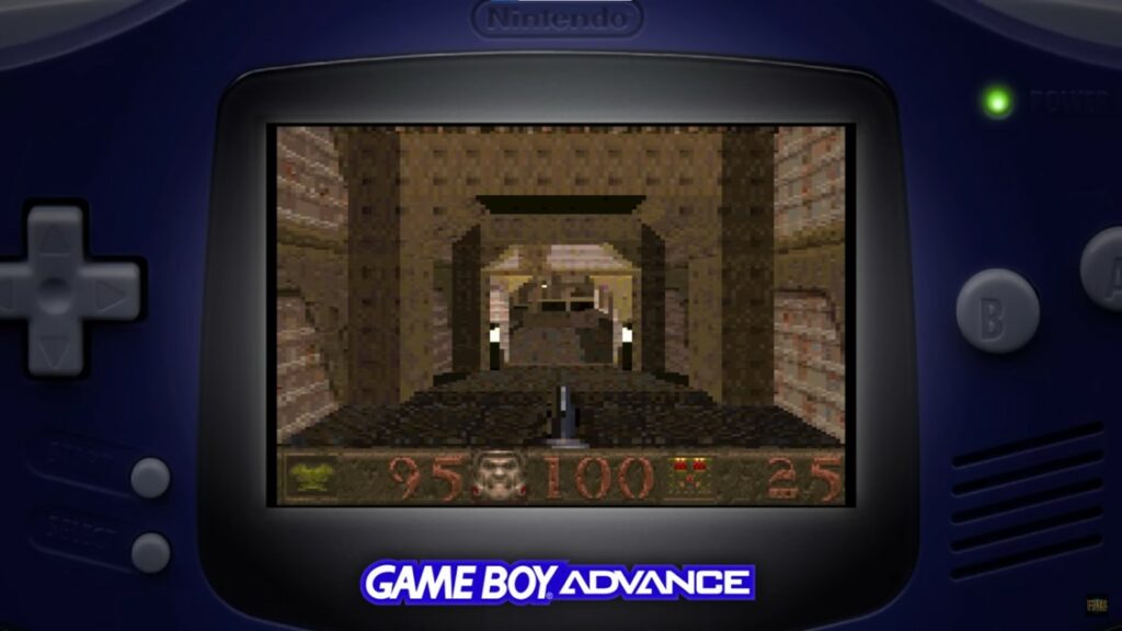
Last year, a video from 2022 appeared on our feeds. It was about a forgotten Quake port to the Gameboy Advanced (GBA). This sounded at least as astonishing as the fake pregnancy tester Doom appeared in 2020, and we won’t hide that we watched the video with a bit of skepticism.
However, closely analyzing the video details and an article we found later, we concluded that, unlike the Doom-on-a-pregnancy-tester, this port was genuine.
The Quake engine was indeed ported, at least partially, to the GBA, a system that is not only slow for Doom’s standards, let alone Quake’s, but also has only 384 kB of RAM, whereas Quake required at least 8 MB of RAM to run.
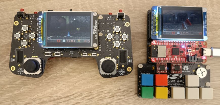
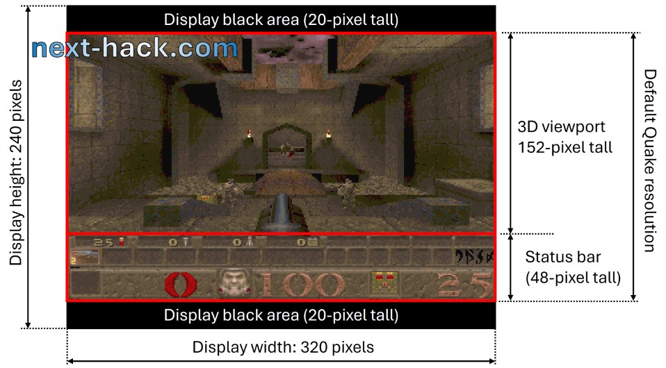
From the video, we understand that the armor count is replaced with the frame rate indicator: 95 means 9.5 fps, and we verified it is accurate. Despite the level of detail is low (the smallest detail is 2 display pixels wide, resulting in only 120×160 pixels actually calculated), and despite enemy AI seems missing (monsters only react if shot), achieving all of this in a 16.7MHz ARM7TDMI, with only 384kB RAM and without FPU is just mind-blowing. This, especially considering that the frame rate sometimes gets quite decent.
This port required much more effort than simply optimizing some member fields in data structures, putting constant data in the memory mapped cartridge, or taking advantage that 120×160 pixels require a very small RAM amount. In fact, from the video and article we understand that this achievement was made possible by almost entirely writing the code in assembly language (the article writes about 200k assembly lines!), and using clever tricks such as, swapping between different CPU modes (e.g., user, interrupt, supervisor) to increase the number of available registers, instead of having to store/load data from RAM.
So far, we have been successfully porting Doom to a number of platforms, and the community ported Doom to many more systems as well. It is now well established that Doom runs on everything that exists (but no, it does not “run” on Escherichia-coli bacteria. The bacteria simply used as pixels of a rudimentary display showing Doom running on some actual hardware, as clearly reported here), so we wanted to find a new challenge. About porting games, of course.
We wanted to find something that was worthy of being ported. Something that was a truly major leap against Doom, in terms of technical advancement. The questions were: what shall we port, and where shall we port it to.
When we realized that someone was able to run Quake – albeit with many limitations – on such small memory amount, we got the answer of “what”.
What about the answer to “Where”?
- We wanted to port Quake using even less RAM than it was done on the GBA (i.e. less than 384kB RAM)
- It would have been nice to use the same microcontroller series we used for Doom, as that would represent a good comparison point. In particular, we wanted to use the same EFR32MG24 series from Silicon Labs or its derivatives (MGM240-series modules, which contain a EFR32MG24). This choice was taken also for two other reasons:
a) We had already some boards running Doom, thanks to the previous Doom port Project, so we could focus on the port, rather than hardware, initially. These boards featured easily replaceable flash ICs, allowing us to install larger ones if necessary (spoiler: we did!).
b) The new Arduino Nano Matter Board uses the same core (MGM240-S instead of MGM240-P), so we could later develop a more advanced DIY handheld console with more pushbuttons, analog joysticks, and better audio.
Wolfenstein 3D, Doom and Quake
In the beginning there was Doom Wolfenstein 3D, probably the first ever commercial first-person shooter. However, due to its technical limitations, it got nowhere as famous and popular as Doom, which is considered the most important and the father of the genre[1].
Despite many fun first-person shooter games that came afterward, it took about 3 years to achieve a breakthrough in the genre: full 3D graphics, including sloped surfaces and floors over floors, with polygonal textured models. This was implemented in Quake, which also featured point dynamic lighting and Gouraud shading for models.
Quake also included a virtual machine, which was able to run bytecode from compiled scripts written in QuakeC, a C-like language developed by John Carmack. This allowed to define the behavior of monsters, triggers, weapons, etc., opening the door to many contributions by the community.
These technical advancements did not come for free.
In fact, on a 486DX @33 MHz with 4 MB RAM you could have a lot of fun with Doom, which could reach a timedemo score of 18 fps on demo3 (according to this and this benchmarks).
To run Quake on the same machine, you needed to upgrade the RAM to 8 MB; however, what you got was more of a slideshow than a game, “running” (we’d rather say “walking”) at just 3.7 fps. (see this benchmark). To reach the same 18 fps time-demo figure at the same resolution, you had to buy a Pentium.
A new challenge, once again!
So, we decided to port Quake, on an MCU, with less memory, the EFR32MG24 series. That was our challenge. Let’s clarify what were our rules and constraints.
- We had to base our port on Id WinQuake C source code (we actually used SDL Quake. The differences are only on the display/audio/input driver).
- The full enemy and game behavior had to be implemented, including all trigger logic, elevators, in-game messages, etc.
- The port had to support all the shareware, including the “start” map where you select the episode and difficulty. (note: as written in the new article this limitation has been lifted, provided you use two 32 MB external flash chips)
- The full graphics engine had to be implemented, including static and dynamic lighting, Gouraud shading for enemies and weapons, animated sky, under water turbulence, mip-mapping, particles, etc.
- Sound was mandatory, supporting ambient, static and dynamic sounds. The sound had to be at least 11025Hz, 8 bit, stereo.
- The status bar had to be the same size as default (48 pixel tall), with full item animation (flashing, etc.)
- Original 320×200 resolution at full details (no pixel doubling), with default height status bar, i.e. 48 pixels.
- No hardware than can offload the MCU was permitted.
- No external RAM could have been added.
The following is the list of what was not mandatory, but it was “nice to have”:
- Quake console, at least in “output”(i.e. printing messages) mode.
- Full save game support (i.e. saving the exact snapshot of the current game, including enemy state).
- Menu/settings.
- Full demo playback support.
The following instead was admitted:
- Any amount of external flash could have been added to store the pak0.pak, the savegames and settings.
- Any amount of overclock was permitted. Overclock just improves playability. Overclocking was also common already back in the 1996 to save some bucks and still have more fun on demanding games. Nowadays, overclocking is also quite common in many hobbyist or hacking projects (such as in many RP2040-based projects).
- Any internal memory regions of the chosen MCU could have been used. In particular, we could use the built-in 20 kB of RAM of the radio subsystem, if we had/wanted to, meaning we had up to 276 kB of RAM in total. We will discuss more in detail later.
- No multiplayer was needed.
- No demo recording support was required.
- No screen size modification: the status bar height and viewport size can be fixed.
- No CD music… Because there is no CD reader!
- If needed, we could have developed any tool to modify the shareware pak0.pak so that it could be optimized for loading and rendering. No reduction in graphic detail was allowed, but all sounds could have been resampled to 8-bit at 11025 Hz..
We admit that this time this project was much, much more complex, and we spent a lot of time for to fulfill all the requirements.
Timeline
The project started in September 2023, when the Doom port to the Sparkfun board was basically done and was requiring just minor changes before publication. This project took quite an effort, and it reached a degree of maturity in April 2024. In the meantime, another project was started, but that’s another story for the future.
The hardware
Initially, we used the same board we developed for the last Doom port.
We made just a couple of changes:
- the external 2×8 MB flash chips were replaced by 2×16 MB ones. This is because the pak0.pak game data file is larger than 16 MB, so it would simply not fit. Noticeably, both flash ICs must have the same size, because we store and read data interleaved to the two chips, to improve bandwidth.
- The audio amplifier gain was increased. This will be explained later but it is counterintuitively related to memory savings. To do this, change R4 to 68 kOhm or even 82 kOhm, and reduce C15 to 68-82 pF (see schematics on previous project).
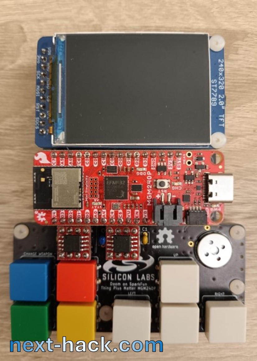
We also developed a brand new opensource board based on the Arduino Nano Matter board. The hardware architecture is the same, but it features the following improvements:
- We added 2 analog joysticks.
- We added 8 more digital pushbuttons (you never know when you run out of them!)
- We used 2 class-D stereo amplifier modules, to have powerful stereo Audio.
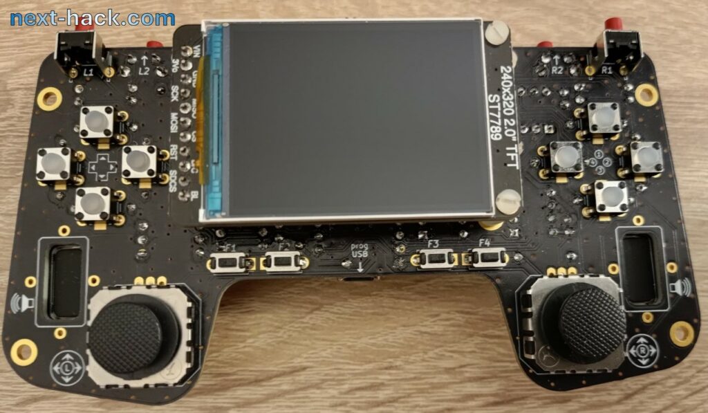
Like the previous one, this board is thought with beginner DIYers in mind, so all the components are through hole (or modules, which do not require SMD soldering). There are two main drawbacks:
- Size, especially thickness.
- Cost.
You are encouraged to design your SMD-only design, to optimize cost and size, based on the design available on the Github repository listed here.
Please note: the design files are provided in the respective repositories, and we do not sell boards/components/kits!
The first impact with code
We used SDLQuake code base, which is exactly as WinQuake plus a couple of source files to support SDL. This choice was made so that we could easily develop in modern Windows releases, having the chance to test and make sure that optimization did not break anything.
Our first reaction when we first analyzed the source was “oh man…”. It was really a very complex piece of code.
There were three different allocators and cache engines, floats and doubles everywhere, huge buffers and, above all, insane stack usage, exceeding hundreds of kB. Ok – we thought – let’s start with something easy!
Our first target was the particle system, because we saw it was very easy to optimize. After few hours of optimization, we were proud of having reduced the particle structure size from 44 to 16 bytes.
But we then realized we were not even scratching the surface…

The challenge seemed infeasible, with too many insurmountable issues and a high risk of failure. We had to take this task with a different view, and not from an engineering perspective. So, we took it as if the porting operation was a game itself: our score was the memory usage. In this case, the lower the score, the better we did, like in a golf match. It was gratifying seeing every time that the consumption was going down. We remember also when we shared our results to our friends:
“We managed to optimize Quake down to 2.5 MB!” “Oh, really? Cool! What is your goal?” “276 kB…”, “still a long way!”.
Well, let memory optimization begin.
256 or 276 kB RAM ?
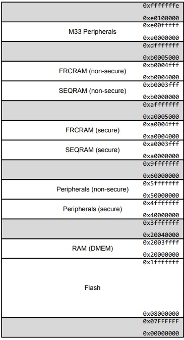
Yes, the EFR32MG24 (the heart of the MGM240 modules) has 256kB main RAM. But it also features a radio coprocessor (a Cortex M0) which also has its dedicated RAM for its low-level operation (Sequencer and frame-rate counter RAM, as described in the datasheet).
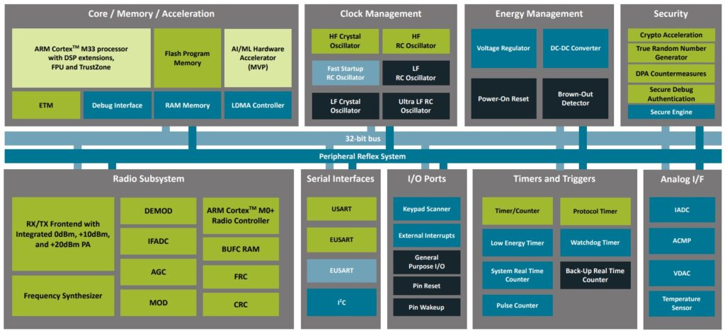
When you are using the radio, such RAM is not available: the radio subsystem is actually a peripheral, like when you connect a BLE dongle or a printer to your PC: they have some internal RAM, but you can’t use it. This is the case of our previous DOOM port: you can’t use such RAM, and such RAM is not even used by the Bluetooth stack, which runs instead in the 256-kB main RAM. The same holds true for the display. The display module has its own (write-only) buffer, but it can’t be used to store anything else, beside the frame to be shown. Instead, the GBA has a memory-mapped display video memory, which can be used as general-purpose RAM to store code or data as well.
In this case, since we are not using the radio subsystem, as suggested by the EFR32MG24 reference manual at page 42, we can use such dedicated 20kB RAM region, so we can have up to 276 kB in total. The drawback is that such 20kB RAM can only feature aligned-accesses and it is also slower, with respect to the 256kB block.

Memory optimization
Quake required 8 MB to run, so it was clear that we had to do an almost impossible optimization job here. The original WinQuake executable is 550kB, which, in an MCU would stay in the internal flash. Therefore, the actual RAM requirement reduces to less than 7.5 MB. In a PC, Quake must load to RAM a big chunk of data, which remains constant. Therefore, like what we did for Doom, we might store to internal flash some data that remains constant, at least during the level, privileging what is accessed randomly and frequently. However, as you see from the github repo, the binary is around 700kB, leaving only 800 kB free. This means that the 7.5 MB figure is now around 6.7 MB. Of that, all the 2D graphics (read: textures) can stay in the external flash.
However, there is still a lot of stuff that is not constant. We will see that such variable data is larger than 1 MB in the original game, as we summarize later. This figure does not even take into account the data that is partially constant and partially variable (e.g. structures, where the almost all the members are constant, but at least one is not. This is the case of model-related structures).
Many of the optimization we made in this project were borrowed from our experience in our last Doom port, so throughout the article we will just briefly mention them.
Old-style optimizations
In this project we used several optimization techniques we already exploited in our previous Doom ports: An (incomplete) list of such old-style optimizations is written below. We recommend to check our last Doom port project for a better understanding.
- Using short pointers (dynamic RAM is always addressed in 4-bytes boundaries, and it is smaller than 256kB, so only 65536 different locations are available, i.e. 16 bits are needed).
- Using array indexes instead of pointers to array elements.
- Trimming data size (e.g. using 13.3 fixed point instead of 32 bits or float).
- Using bitfields.
- Optimizing memory allocator.
- Using bitfield arrays to determine whether a node/leaf is already marked as visible instead of a 32 bit frame counter. This was also used in Doom.
- All constant tables/arrays are kept in flash.
- Separation between constant and variable data from structures. If a structure contains both constant and variable data, these were split into two different ones, one which stays in flash, the other is in RAM.
- Caching to flash. This can be both related to game data (e.g. level geometry) or to arrays, which are calculated at runtime and then stored to flash as they are constant for the whole level duration. For instance, this is the case of the “mod_known” array, where the pointers are constant, after all the models have been loaded.
Noticeably, this time not only we had to optimize data stored in RAM, but also the one that is stored in internal flash. In fact, for speed reasons, we would like to put as much constant data as possible into the internal flash, because it much faster than external flash[2]. The more compact is the data to be stored, the more the data that can be later read faster.
However, we had to take a tradeoff between internal flash memory savings and speed. In fact, some 3D model data structures are used frequently during rendering, therefore their access should be as fast as possible. Using packed structures or even worse bitfields, or even just having a structure whose size is not a power of two, could slow down some accesses or pointer operations. Therefore, for selected structures, we preferred speed optimization, if we found that we could afford it.
For instance, when we found we had enough spare flash, we preferred keeping a structure size to a power of two, so that pointer operations were faster (e.g. getting the index of an element in an array knowing the pointer to such element). When this would not have been possible without sacrificing too much memory, we still tried to optimize some members for speed, by not using bitfields.
In some cases, to improve both speed and memory optimization, we split structures in two separate ones, so that each one was a power of two. That’s the case of the espan_t structure, which was split into one 4-bytes long structure and one containing only one byte. Using a single structure would have yielded a 5-byte packed struct, which would have impacted too much speed. Noticeably, the original e_span structure was 16-bytes large.
Finally, optimizing data in external flash also has its benefits. For instance, if an array of 32-bit integer can be replaced with 16-bit values, then we can cut in half the slow load time from external flash. In the original Quake, 32 bit integers were used extensively, because on a 32 bit machine they are much easier to handle, and loading from RAM a 16 bit or a 32 bit value takes the same amount of time, if it is aligned. Yes, we have a 32-bit machine as well, but reducing transfers from external flash brings more benefits than using always 32-bit integers.
Display Buffer
In the previous Doom port, we had so much memory that we had the luxury of using a double buffer for drawing: while the DMA is sending one buffer to the display, we can write to the other. At the end of the frame (and DMA operation) we swap the role of the two buffers.
This time, not only we cannot have a double buffer, but also, we can’t even afford a single one!
Luckily, the 3D viewport is only 320×152 pixels: we can draw the 3D scene first, and then the status bar.
Z-Buffer
The memory scarcity problem is exacerbated by the requirement of the z-buffer.
What is the z-buffer? It is a buffer storing the distance between the screen (your eyes) and each pixel: in other words, it contains the z-coordinates of each on-screen pixel (actually, Quake stores the reciprocal of the z-coordinate).
Why do we need it? When drawing the 3D scene, some objects are not drawn in order of distance. This is the case of “alias-models” (i.e. enemies, and some bonuses). Therefore, we need to determine whether the pixel we want to draw is closer to the screen (i.e., if it will be visible) compared to the one that has already been drawn. If it is not, we won’t draw it.
Noticeably, Doom did not require z-buffer, because the walls are always vertical, sprites are drawn in back to front order and all the pixels of a sprite have the same distance. This does not hold true anymore in Quake, as, for instance, each model can have pixels both closer or farther with respect to already drawn ones, because models are now 3D and not flat.
The 3D viewport is 320×152 pixels, which means that 97280 bytes are used by the z-buffer alone, because each z-buffer element is 16-bit wide.
Display: the whole scenario
To the previously mentioned z-buffer, we have to add the actual frame buffer, which we already said to be only 320×152 bytes, because we exclude the status-bar, which can be rendered and drawn later.
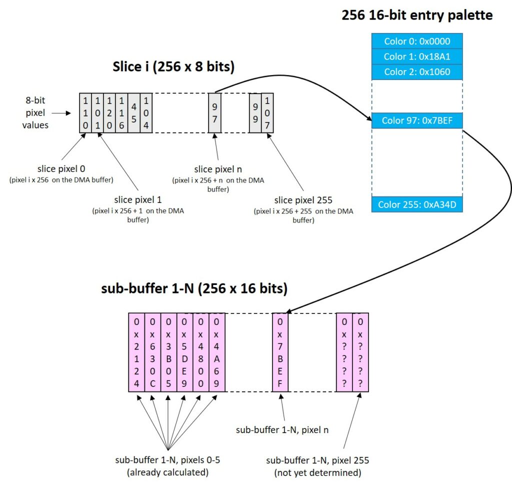
This brings the total memory occupied just by the display to 145920 bytes, i.e. more than half of what we have in our system. To this amount, we need to add 1kB, for on-the-fly 8-to-16 bit conversion, as we did in the Doom port: we convert 256 8-bit pixels to 16-bit pixels and we send to DMA. Just after we start a DMA transfer, we prepare another 256-pixel block, so that the block will be available before we have to start next DMA operation. This repeats until the whole frame is refreshed. For this, we need two small buffers of 512 bytes, i.e. 1kByte. The total is about 147000 bytes (143.5 kB).
RAM re-usage
The most attentive or expert reader might have already realized that the 97kB z-buffer would be used only during 3D scene rendering: this would be a huge waste of memory. That’s why, after the scene is rendered, we use the last 48*320 bytes of the z-buffer to draw the status bar or bottom part of the menu or console. This allows to immediately start rendering the top part of the screen even when the DMA is still sending the first bytes of the status bar, speeding up everything.
This is possible because the first part of the rendering process involves drawing the world model surfaces on a row-by-row basis, from the top (y-coordinate 0) to the bottom (y-coordinate 151).
This is neither the only occurrence we reuse the z-buffer, nor the only buffer we reuse. Beside the z-buffer, we reuse another smaller buffer we will talk about later: the “texture cache buffer”. Later, we will cover this smaller buffer and further explore how the z-buffer is reused. In the picture below, we illustrate the extent to which we are reusing memory that would otherwise remain unused for most of the time.
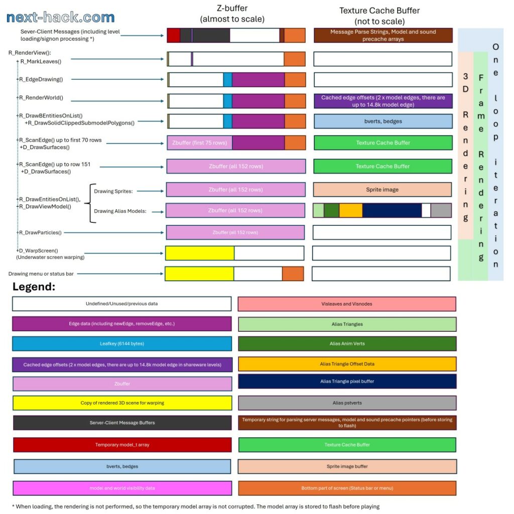
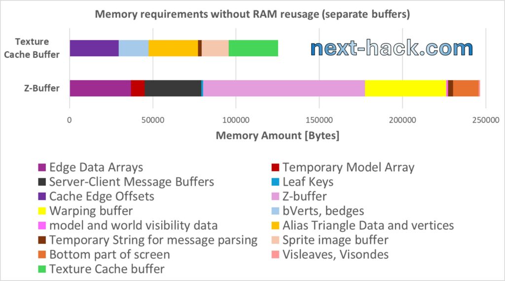
As you might notice, each buffer shown above is reused multiple times for different temporary data. In particular, we reuse each buffer between 2.5 and 4 times. Their combined size of 124 kB allows us accomplish what would require 373 kB of RAM if we used separate buffers for each purpose
Note that in the picture above, the texture cache buffer is less than 1/3 the z-buffer, and, while the z-buffer division is drawn almost to scale, the buffers in the texture cache buffer are not. This is because many of the buffers allocated in the texture cache buffer do not have a fixed size.
In the picture below, we show for each buffer, how much temporary data we used it for.
Three allocators?
Quake uses 3 allocators (actually 4, as malloc is used as well) to handle memory and to cache objects.
The first allocator is the hunk, and it is the most complex. It allows to allocate memory and cache data. When freeing one chunk of memory, it allows for repacking, so that the memory fragmentation issue is prevented.
The second allocator is a somewhat reduced version of something we have been used with in Doom: the zone memory. For the zone memory, Quake allocates about 50kB and it is used for frequent allocation of small buffers such as texts used for instance for the console. It is also used to register the “cvars” (console variables) and the console commands.
The third one is the surface cache buffer.
We have removed the hunk and the surface cache, and we replaced the zone buffer with an optimized version of what we used in our Doom port. In fact, in MG24 Doom, the block overhead was 8 bytes per block, mainly because we wanted to use memory pools and there was a member called “user pointer”. As we will explain later, in this port we won’t be using memory pools, therefore the block overhead is reduced to only 4 bytes. The drawback is that we can’t have a memory zone larger than 128kB, but this is not going to limit us: we won’t have the opportunity of dedicating such large amount of RAM to the zone memory.
Noticeably, the role of our zone memory is different to what the original Quake uses it for: as we will explain later, we mainly use it to allocate monsters, projectiles, bonuses, etc.
Trimming limits
In the Quake code there are some hard limits defining for instance how many objects, models, sounds, etc. there can be. These were set to a relatively large value so that modders could have had a relatively large freedom to add features, create more complex maps, with more enemies and bonuses. This is beyond our scope (which is to run the shareware Quake), therefore we have analyzed all the shareware levels and we have trimmed the limits so that we have just a reasonable safety margin to run the shareware episode.
One might wonder why we added a safety margin, if we profiled all the maps. The reason is that, while some things like number of nodes is static (i.e. they depend only on level map data), other are not. For instance, the number of on-screen visible surfaces strongly depends on your location, and what you are looking at. We have logged such numbers during actual gameplay, which is not something 100% reproducible (monster behavior is random, and player position and direction have close to infinite possibilities, etc.).
Also, Quake allows to specify how many particles can be used, from a minimum value of 512. 2048 is the default value, but we chose the minimum for sake of memory occupation (each particle structure is now 16 bytes long, and 512 of them still require 8kB RAM).
Stack you very much
The first time we saw the R_RenderView_ () function, we were, let’s say, a little bit… surprised:
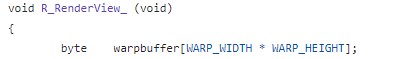
Yes, a 64000-byte buffer was allocated on the stack, for creating the underwater distortion effect (warp). This is done essentially by telling the renderer to put the rendered pixels in that temporary stack buffer instead of the regular frame buffer. Then, such buffer is copy-distorted to the regular one.
To save these 64000 bytes, we render on the regular framebuffer, then we copy the buffer to the (now unused) z-buffer, and then we do warp-copy from there. This savings comes at the expense of the additional copy to z-buffer operation.
However, this was just the tip of the iceberg. A much bigger stack usage was coming from the 3D renderer. In fact, Quake uses the leading edge renderer technique, which requires to keep track of polygon edges, corresponding to the surfaces to be drawn. An algorithm will find which edge/surface is on top of the others. For each row of the 3D viewport, the surfaces are rasterized into spans. Each span is a horizontal line of consecutive pixels belonging to the same surface. The surface will typically extend vertically for many pixels, so these spans form a linked list, while the surface points only to the first span in the list.
In each frame there might be many hundreds of surface span and edges, and these are statically (i.e. the array size is fixed) allocated in the stack, requiring more than one hundred kB. For instance in the function R_EdgeDrawing(), two arrays are allocated in the stack.
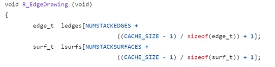
The original sizes of edge_t and surf_t are 32 and 64 bytes, respectively. By neglecting the additional CACHE_SIZE part, knowing that the original NUMSTACKEDGES and NUMSTACKSURFACES are 2400 and 800, respectively, this brings the total stack usage, just for this function, to 128000 bytes. The function then calls R_ScanEdges(), which use 3000 (MAXSPANS) espan_t, each one being originally 16-bytes large, adding 48000 more bytes.
To solve this issue, we acted in different directions.
First, we analyzed and trimmed limits as previously discussed.
Second, each data structure was trimmed to occupy just as many bytes as needed. This yielded even more savings than the trimming limits.
Still, even with this, we would have needed (just for the function R_EdgeDrawing()) at least 60kB stack.
To cut in half stack size requirement we used once again the z-buffer. In fact, even counting that the last 15kB are later used for the bottom part of the display (which might still being sent during the surface rendering), we have a lot of kB left: 80kB.
To understand which data we put in the z-buffer array, we need to clarify how rendering is done[4].
To draw surfaces, the following steps need to be done:
- determine which edges and surfaces are present in the frame (including determining which are the surface closest to the screen).
- using the active edge lists, generate spans for each screen line (scanning from row 0 to 151), and associate them to the surface.
- for each surface, draw the associated spans.
You’ll recognize that in step 3 we don’t need edges anymore. For this reason, we split the surface rendering process into two approximately equal regions in size, and we store the edges (ledge array in R_EdgeDrawing()) just before the region we use for the status bar or bottom part of the display, in the z-buffer (see picture about RAM reuse).
When we render the surfaces of the first half of the 3D scene, we are not corrupting the edge data stored in the z-buffer, because at most we are writing to the first half of the z-buffer.
Then, we compute the spans for the second part of the display, reusing the same span array we used before. When we need to draw such spans, we can safely write to the second half of the z-buffer because:
a) edge lists are not required for span drawing, once span data have been generated.
b) typically, when the first spans have been actually drawn, the DMA has already finished sending the whole data to the display. In some cases, this is not true, especially when facing a wall, i.e. very fast rendering. To exclude unwanted artifacts, before starting the rendering of the second part of the 3D scene, we wait for the completion of the DMA operation.
You might wonder why, when we are rendering the spans, we render before the first 75 rows, and then later we render the remaining 77. Wouldn’t have been better splitting equally?
Yes, it would have. However, there was not enough memory for that. When we draw the first rows (in this case 75) we still have to keep the edge information for the remaining 77 rows.
Noticeably, the number of “spans” that can be calculated for each pass is limited to MAX_SPANS (defined in r_shared.h). In the original Quake code, this value was set to 3000, which did not pose an actual limitation because the number of “passes” was not restricted to 2, as it is now. We cannot perform more than two passes because, after the second pass, the edge list is overwritten. For this reason, we increased MAX_SPANS to 3500. This change does not represent an increase in memory usage compared to the original code, as we use only 5 bytes (4 + 1 in two separate arrays to improve speed) per span, instead of 16.
We also used static stack analysis to identify opportunities for optimizing stack usage. For instance, Quake utilizes large buffers on the stack to store temporary strings. We realized that this occurs when the z-buffer or the texture cache buffer is not used, so we placed such strings there, allowing us to reduce the space dedicated to the stack and use it for other purposes.
Server-Client
Quake takes a very different approach than Doom, when it comes to the game-logic. In Doom, regardless of whether a single or multiplayer game is started, each client/host always runs the physics/game logic engine locally, which consumes the user and other clients’ inputs. In other words, even when playing a multiplayer game, you are playing a single player one, with the difference you are sending to the other peers your inputs, and you are getting theirs from them. This works because in Doom, given the same inputs from all players, everything is 100% reproducible, due to usage of pseudo-random numbers, which are initialized with the same seed at the beginning of the match. This of course requires that all the clients/host have the same code and the same WAD file.
Instead, Quake is split into two parts: a client, responsible of reading input, sending/reading to server, and render the 3D scene, and a server, responsible for physics, hosting the actual game, and communicating with clients. When Quake is not hosting a game, i.e. during demo or when joining a remote game, only the client part runs. Instead, the server part runs as well when we are playing a single or hosting a multiplayer game.
This solution was probably taken as it eases addition of multiplayer using different communication interfaces (serial, TCP, etc.), and also prevents demo desync, which was a plague in different Doom ports, requiring a lot of efforts to fix them.
Unfortunately, this choice comes with a huge memory footprint (for a MCU with few hundreds kB RAM).
- You need many large buffers (around 1-8kB each), to store server-client messages, even if these are sent in loopback. These buffers require over 32kB in total during a single player game. Yes, we could have completely rewritten the code so that no such buffers are used, but it would have taken us a lot of time (however, we did change the code only for server-to-client entity status update, as we will discuss later). It was much easier to realize that in a single player match, all these buffers are consumed before the client renders the scene. This means just one thing: we can use the z-buffer to temporarily store the server-client messages, as you might have seen from the figure about memory reuse.
- When playing a single-player game, there is a lot of duplicate data between server and client, pertaining to objects such as monsters, doors, bonuses, etc. We talk about this in the following section.
Edict and entities
The server-side keeps all the parameters of each object (monster, player, bonuses, trigger, door, etc.), including position, frame, state etc. These were stored in an array of structures called edicts. Since the game was made so that an edict could have been “anything”, e.g. a monster, a bonus, or a door, the original edict_t structure included all the possible properties and handlers for all kind of object. This had the drawback that the structure size was around 800 bytes.
The client side needs to know some information of each object for rendering, such as their frames, positions, etc.
This is actually duplicate data, if you are playing a single game match, because they are related to what is stored in the edicts.
Objects in the client-side are called “entities” (entity_t structure), and there were stored in 3 arrays, depending on their type: client, static and temporary entities. The entity_t structure was 180 bytes large.
Unfortunately, we cannot use chose just one or the other, we had to support both.
For instance, entities contain some information which are not present in edicts. Entities are also needed for demos. Demos are very useful benchmark and regression testing tools, so we did not want to just drop demo support.
On the other side, Edicts contain a lot of information not required for rendering, but for the physics/game logic engine.
Therefore, we used the following strategy:
- We have “removed” static entities (we will discuss about this later)
- We have created a generalized entity, which contains:
- a field specifying the entity type (edict, temp entity or client entity)
- some rendering information missing on the edict (e.g. topnode)
- a pointer to the entity data: if we are in a live game it can be edict or temp entity, if we are playing back a demo, it can be a client entity or temp entity.
- we have created getters and setters to be used by the client, to retrieve the data, such as angle or position. Based on the entity type the getter will fetch the data from the correct entity array, or from the edicts. There are two entity arrays. The first one is the client entity array, used only during demo. If the demo is playing a big array is allocated in the zone memory, taking 32kB (after optimization). This array is freed as soon as the demo is stopped, because during actual gameplay, the zone memory is used by edicts. The second type of entities is temp entities, used to show, for instance, the beam of the lighting gun, or the gun itself. This array is static.
In the original game, edicts were statically allocated in a huge array of 600 elements. We have verified that in shareware game this can be safely reduced to 400 units. Still, this was far from enough. As mentioned above, an original edict contained all the possible data to hold all the information of any possible thing, regardless of its type: a light, a rocket, a door or a monster. This resulted into a huge edict size, about 800 bytes, amounting to 320kB even using only 400 of them (480 kB using the original limit). Since Quake also used the entities, together with edicts, and since each entity occupied about 180 bytes, the consumption was around 600 kB, or 400kB with trimming.
To reduce such enormous amount of RAM, we have listed all the possible “things” (projectiles, doors, triggers, enemies, lights, etc. There are about 100 of them.) and we have grouped them into classes (not C++ classes. Here we mean class of objects). Each class just features those fields that are actually used in the game for that particular type. For instance, a static light won’t have speed, angular speed, etc.
All the edicts have a common part (which contains the object type, the short pointer to next edict, the “used” flag, and the area information), and a class-dependent structure, containing all the class-specific properties and handlers. We have developed a tool, which generates automatically getters and setters for all the class types based on a configuration array (for each entity type and for each field, it determines the level of implementation). To understand which field/handlers were needed, we both analyzed the Quake C code (we will discuss about that later) and we played each level (an error was thrown if an unsupported field was used). Of course we had to modify the code so that instead of accessing directly to the original field, the getter/setter function is called. This, based on the edict class type, will call the correct implementation and return the data, regardless of how it is stored.
Each member field of each class was also later manually optimized to reduce the number of bits used. This allowed to cut down memory requirement for all edicts at the worst condition well below 40kB.
Since the edicts are now with different sizes, these can’t be stored in an array anymore, so these are dynamically allocated.
Entities also had efrags, which were used only to draw static entities, we mentioned before. Static entities are those entities that play no role in the gameplay, and are animated locally, i.e. on the client side. Example of static entities are torches. Static entities were introduced in the original Quake probably to offload the server-side calculation and reduce the number of edicts. There are at least two ways of getting rid of efrags, both involving removing efrags and the code associated with them.
- Let “makestatic() function” to be a stub function. This has the side effects that, for instance, torches won’t be visible in demos. These will still be visible and animated in a live game.
- Add to the client entities an “entleaves” array, which contain the information about which world leaves the object is touching (for a better understanding about leaves, we suggest you watching videos in the references). This is filled when the edict is declared as static calling makestatic(), and then the array is stored to flash (as well as other static data). It is also filled, during demo playback, when the CL_ParseStatic() function is called. There, the function CL_FindTouchedLeafs() function is called, to find the leaves touching the entity. We created this function based on the server-side SV_FindTouchedLeafs() (yes, we used the same “leafs” word).
When playing back a demo, in R_RenderView_(), after MarkLeaves()—which identifies the potentially visible leaves—we check each static entity to determine if any of the leaves it touches are potentially visible. If so, the entity is added to the visible list. Notably, this solution will increase the size of the client_entity by 16 bytes, making each one 80 bytes in total. Consequently, the corresponding 400-element array will occupy 32 kB instead of 25.6 kB. This increase is not a significant issue, as the Z memory usage is very low during demo playback. Yes, we could have restored the static entity, putting only there the additional entleaves structure, and saving some bytes. However, we found that the simpler solution runs efficiently, and further optimization is unnecessary.
Note that in both cases, torches and other static lights will be calculated as regular entities at server side, i.e. in a live single player game. Initially we used option 1, but later we switched to 2, because we wanted the demo to be 100% faithful, for a fair, apple-by-apple benchmark with online-available data.
At this point, it is worthwhile to discuss a pending issue that we left unaddressed: how we modified the server-to-client visible entity data communication.
We have already mentioned that during a match, the server shares a considerable amount of data with the client. In the original code, the server checked each object to determine whether it was potentially visible to the client. If it was, the server sent a status update containing information about the parameters (e.g., position, angle, frame, etc.) that had changed since the previous frame.
Instead, we now store information about which objects are potentially visible to a single local player in an array of bitfields. This approach uses only 50 bytes, as we limit the maximum number of objects per level to 400 and use a single bit for each object. Access to this array is shared by both the server and the client. Therefore, during a single-player match, the client does not need to parse a packet to retrieve entity information, as is required during demo playback; it simply checks whether an entity is visible. If it is visible, the data is directly fetched from the edict entry using the getter function.
Finally, we want to explain now why we did not use memory pools in our optimized allocator, as we did instead in Doom. In our last Doom port there were only 3 classes. Full, partially static, and fully static objects, so there were only 3 pools. Instead, we have many classes here, to minimize object size. The edict size is now variable, so we need as many pools as the number of classes, which is, at the moment of writing, 22. The size of each edict varies a lot, and it is between few bytes up to some hundreds. To understand why using pools is a bad idea, let’s consider an example of edict size of 80 bytes, and a pool size of 8 elements.
With a pool size of 8, the allocator overhead would be 1 bytes/object (because the allocator overhead would occupy 8 bytes, but each pool can store up-to 8 objects). If we allocate 400 objects of 80 bytes, we would waste 400 bytes in overhead. This would be 1600 bytes without using the memory pool, as each object would have a 4 byte overhead.
Now let’s consider the case that there is a pool not completely filled, and it has just 1 object. We are allocating 640 bytes (+ 8 overhead) to store only 80 bytes. We have wasted already 560 bytes. The case without pools is still worse, but we don’t have just one pool, we must consider 1 pool per class type.
So, let’s now consider that we don’t have only 1 pool type, but 22 pool types. In the worst case we are wasting 7 multiplied by the sum of the sizes of all the object types. There are 22 classes, so 22 pool types, and let’s suppose the average object size is 80 bytes. This means that 7x80x22 B (about 12kB) might be wasted due to not fully used pools in the worst case, vs only 1600 bytes. The same would hold true even if the average object size would be much smaller, i.e. 32 bytes. We would waste about 5kB instead of 1.6 kB.
Sky
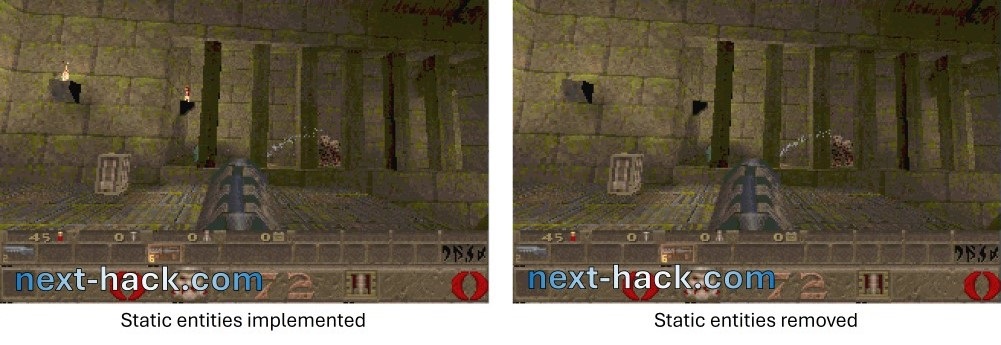
In Quake, skies are generated by overlapping two layers. The bottom layer is partially transparent, and it moves with respect to the top one. The resulting combination of top and bottom layers moves as well. This creates a nice animated sky with parallax.
For this effect Quake used about 64kB RAM. Since the texture is a square 128 pixel large, and since relative direction is fixed, we have decided to prerender all the 128 possible frames in the pak0.pak. This means that for each different sky, the pak0.pak increases of 2MB. In the shareware pak0.pak there are only 2 unique skies, so the size increases by 4MB, which is affordable, as we have 32 MB external flash, and the original pak0.pak is less than 20 MB.
This solution not only reduces RAM usage, but also increases speed. In fact, instead of using 48 kB RAM, and recalculating the sky frame, we just load from external flash the correct sky frame to be drawn (this takes less than 1ms on the overclocked MCU).
Surface cache buffer
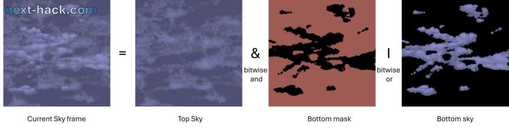
Quake used a clever strategy for lighting surfaces. Gouraud shading was not used for surfaces, because it is vertex based: light is calculated at the vertex of each surface, and then it is linearly distributed for the internal pixels of the face. This has the drawback that for large surfaces, the lighting details would be poor. A solution to this problem would have been to split large surfaces into smaller ones, increasing rendering time and memory usage.
John Carmack came out with a clever idea: a 16×16 pixel grid is logically applied to each surface. Each point of that grid contains the light intensity of that particular surface pixel, and it is called “lightmap”, which is calculated at level-editing time. The contributions of dynamic lights are added to each point of this lightmap and temporarily stored into the “blocklights” array, which contains the total light of each point of the grid. The light level of the internal pixels of those 16×16 squares is calculated by bilinear interpolation, taking the values from the vertices.
Noticeably, on-the-fly bilinear interpolation is rather CPU-intensive, so Carmack’s idea was to implement a surface cache. Once the engine determines a surface needs to be drawn on-screen, it prerender it into the surface cache, before using it as texture for the world model face. The next frame will very likely contain the same pre-lighted surface: if the surface cache still contains said surface, no costly lighting calculation is required again. The surface cache was large enough, therefore, for each frame, none to few surfaces must be pre-lighted, as they are already available in the cache. When there are dynamic lights (or flashing light effects) the surface must pre-lighted again. However:
- dynamic lighting or light change effects occurs relatively sporadically.
- dynamic lighting effect are limited in space, so it will affect a small fraction of the cached surfaces.
Remarkably, although in general bilinear interpolation is a costly operation, in the original Quake code it is implemented incrementally on the whole surface, reusing previously calculated data, amortizing the complexity by a factor of 16.
All of this cannot be done in our case.
The default surface cache size was 600kB for 320×200 resolution, even though we profiled that the surface buffer might be as small as 250kB-300kB, just to hold all the surfaces in a single frame. This was still too much, so the surface cache was removed completely.
Initially, in its place, we implemented a single surface buffer: every time we loaded a texture to the small surface buffer, we tile and calculated the lighting for each pixel, and then we used the buffer for rendering. Such buffer was around 32kB in size. If a surface was larger, its mipmap level was increased until it fitted into the 32kB buffer. Noticeably force mipmap increase occurs very sporadically, and it is very hard to spot when it happens.
Later on, to improve speed (and collaterally, graphics details and memory usage as well), we implemented the texture cache buffer, which will be discussed in the speed optimization section.
Quake C
Quake gave the opportunity to modders to express their creativity not only by allowing custom maps and graphics to be created, but also it allowed to change monster’s behaviors, game logic, triggers, and (partially) physics. This was achieved through the Quake C scripting language. This language is very similar to C, although it has several limitations, we are not discussing here. The Quake-C files are fed to the Quake-C Compiler (QCC), which creates a bytecode. Such bytecode (progs.dat) is loaded in RAM and interpreted from there.
Such customizability feature is far beyond the scope of this project, but we still wanted to implement the 100% of the shareware quake behavior, so in a way or in another, such code had to be included.
We thought that interpreted code had some disadvantages.
- It requires to load into RAM a huge chunk of data, which is more than 410kB. Yes, we could have copied it to the internal flash or even left in the external one. Putting the bytecode into the internal flash means that we will have 410kB less for frequently used data such as world-model data. This is a no-go, as we will see later. Leaving it into the external flash requires to implement some caching algorithm. As conditional execution/jump/branches are very frequent in the Quake C code, this would have resulted in frequent (slow) load from external flash.
- Some additional RAM (about 2 kB) is required to run the virtual machine.
- Each low-level instruction takes 12 bytes, and unlike the GCC compiler, QCC does not have optimization options, so we expect the bytecode to be larger.
- Emulated code is slower than running native compiled code.
What we wanted was to translate the Quake C code into a native C code. We could not have done it manually, as all the files count for more than 16000 lines of code. We wanted to apply only minimal changes if needed (spoiler: we had to).
Therefore, we used the Quake C compiler code base and converted it into a Quake C to C translator. The Quake C code is translated in a way so that edict members are accessed through getters and setters, to take into account that each edict can have its sets of members, depending on the class type (monster, player, door, etc.).
Of the 16 thousands lines of Quake C code, we had to modify a few (about 30 around various files, plus about 100 in defs.qc to define class names, but these were copy and pasted from a spreadsheet).
In particular, our Quake C to C converter requires that each function must be declared or implemented before it is used, otherwise spectacularly nasty bugs will occur. Other changes were made to fix potential bugs or warnings in the original qc files (such as functions not returning a value). These changes have been marked.
Secondly, when the spawn() function is called, the original Quake used one big edict element, regardless what will be used for, e.g. missile, bonus or monster. In our case, we need to specify which class type will be the spawned object, so we must pass it as argument to spawn(). Therefore, we had to search for all the spawn() calls in the QC files, and insert the class type of the desired object to be spawned.
Sound
Sound was optimized by removing redundant data from the channel and sound structures, as well as trimming their field sizes. For instance, the sound.h files defines the following structures:
- sfx_t, which contains the sound name and its cache entry.
- sfxcache_t, which includes the sound data and parameters (e.g. length, rate, start of loop, if it is stereo, etc.) The length of this is 20 bytes plus the actual sound sample data.
- channel_t, containing the status of a channel. This structure is 52 bytes long
The sfx_t structure has been modified. It still contains the sound name, but also contains the length, loop start position and a pointer to external flash, where sound data can be found. The array of sfx_t describing each sample is stored to flash when all the audio data is parsed.
The sfxcache_t structure is not used anymore, while the channel_t has been optimized to 16 bytes, and the array of channel_t must stay in RAM as everything here now is variable.
The low-level sound engine was partially borrowed from our previous DOOM port, and partially rewritten to be compatible with the original Quake higher level implementation.
Noticeably, in Doom we used a 16-bit audio buffer, because the DAC is 12-bit. To save some kB we are using an 8-bit buffer. Unfortunately, the DAC does not allow to set up a 8-bit mode, so the signal will have a voltage which is 1/16 of what it was achievable in Doom. This means that the sound power would be 1/256, i.e. very quiet. For this reason, some resistor values need to be changed to restore the full volume in the Sparkfun-based board. In “The Gamepad” board, we did not put any amplifiers[3], and the Class-D amplifier can only amplify at most by 16. This would yield less than 0.3W. Therefore, for “The Gamepad” configuration we opted for high speed 8-bit PWM. If you use DAC, the audio will be very quiet. You can increase the power by 6 dB by changing the input resistor values R5 and R6 to something much smaller, like 330-100 Ohm, still, we believe that the sound level will be very low.
The full sets of sounds are supported: static (i.e. when going close to a burning torch), ambient (i.e. water effect) and dynamic ones (i.e. weapon noise, etc).
Console, CVars and Commands
The console was an iconic feature of Quake. Indeed, the game starts by showing it. The console allows for several debug features (which we used a lot in the PC side) and allows to enter cheats as well.
However, the console, command handling, and CVars (console variables) required a lot of kB of RAM. Since we expect that in the MG24 port nobody is going to perform directly debug operations, we reduced the console buffer to basically being able to hold only one screen worth of data (about 1kB), instead of 16384 characters (about 16 pages). History was eliminated and, in its place, we put a list of hardcoded cheat commands. Pressing up or down in console mode will bring into the console line the next cheat code, which can be then entered pressing fire.
CVars were also implemented quite in an expensive way, by registering them at runtime, and using a float to store even Boolean flags. There are tens of such variables, and the Cvar structure was 24 bytes large. Noticeably, CVars were dynamically allocated in the Z-zone, requiring therefore an additional overhead. Such overhead would have been 4 bytes with our optimized allocator, and much more with the original one.
We could not simply have removed them, because these are used extensively in the game. Therefore, we removed all the calls that register these variables and put all the variable declarations in a big constant array, which contains:
- the type of variable (float, short, string, int, etc.)
- the pointer to that variable
- the variable string name.
- the string corresponding to initial value.
- the features of the variable (e.g. if we must store them as game settings).
Noticeably, we introduced the limitation that string variables are constant, but this was not an issue for the game, at least in the shareware version. All the other variables can be changed.
In this way, the new RAM occupation for each Cvar is 4 (float or int) or 2 (short) o1 byte only.
Similarly, in the original code, console commands were dynamically registered at runtime with the Cmd_AddCommand() function, which registers a cmd_function_t structure into the hunk region. Such structure is 12 bytes large, excluding the allocator overhead. Similarly to what we did for Cvars, we register all the commands at compile time, in a constant array.
Keyboard
The keyboard also used a lot of RAM. The arrays that are constant throughout the game have been pre-calculated and put into constant ones, which stay in flash. Also, the game uses an array to keep the key-pressed state, one byte per key. This has been put in a bitfield array. Key bindings were also optimized, while maintaining the possibility of remapping controls.
Caching to Flash
Caching to flash has been done in our previous Doom ports, and we have discussed extensively in the previous articles. Caching to flash is of fundamental importance to improve speed, especially for those data which is accessed with random order. There was not enough space for any kind of texture data, so we gave priority to world mode data (faces, nodes, etc.). Other things, such as even some alias-model animation data, triangle data and all the graphics content are fetched from the external flash: these are loaded to some RAM buffers when needed. Such buffers are temporarily located into the texture cache buffer.
Noticeably, caching to flash has two big drawbacks:
- Level switching takes a lot of time, about 12-13 seconds.
- Caching to flash will wear it out. In fact, if the data is different, the page it will be stored to will be erased, and programmed with the correct values. The MCU flash has an endurance of 10k program-erase cycles, which means that the reliability will decrease after 10k cycles. The datasheet does not state what occurs after 10k cycles, but we might guess that the retention won’t be the specified 10-year time anymore, or there might be some stuck or erratic bits. We don’t think that such bits will occur abruptly after 10k cycles though. Also, even if you leave the demo sequence running, it will take approximately 10000 minutes to wear the flash out, which means you are leaving the device powered on for about 7 days. That’s why we suggest to disable demo playback by editing in quakedef.h the “ENABLE_DEMO” to 0.
Particles
We have already mentioned them before, and we will briefly cite the optimizations we used:
- Coordinates were changed from float to 13.3 fixed point. Velocities had even smaller size.
- Lot of bitfields usage. For instance, instead of storing a value explicitly, we store use a small number of bits that make the index to a constant array storing the particular value.
- Particles were in a linked list, so they required a “next” pointer. Now they are in an array, so no next pointer is required.
Strings
Generally, literal strings in C do not use RAM; the compiler recognizes them as constant arrays, so they are stored in flash memory. However, in our case, we must consider the following:
- In our code, we refer to Quake C strings by their index. The strings are all collected into some arrays, and to use them, you must provide the index to the function getStringFromIndex(), which returns the corresponding constant string. Since there is more than one array, the indexes are divided into ranges, with each range associated with a different array.
- The ‘PAK’ file contains many strings that are not present in the QuakeC code. As a result, these strings are not automatically included in an array within the autogenerated C files created by our QuakeCConverter utility. This complicates things significantly when, for instance, Quake needs to print a message if the player activates a trigger. In this case, when Quake parses the level data, it must associate the message with an index that will later be used by getStringFromIndex() to retrieve the string value. However, this string is not stored in the internal flash; it is only available on the external flash.
To fix this issue, in the utility we use to convert the PAK0.PAK file, we also print all the strings found in the level data. These strings must be included in a constant array in pakStrings.h. When we parse the entity data of a map, we obtain the corresponding index from the string in the BSP file through a simple string search in the pakStrings[] array. Later, when Quake needs to print the message, it provides the same index, and the getStringFromIndex() function recognizes that this index refers to pakStrings[]. It then subtracts an offset to retrieve the string from that array.
Speed Optimization
We must admit that the first time we managed to have the demo1 “running” on our device we were amazed by the fact we reached this milestone: the full 3D engine was running on only 276kB RAM! Still, we were also prepared to face the truth: the port was running extremely slow, between 4 and 6 fps. As a matter of fact, we expected even worse performance, e.g. 1-2 fps.
We also already knew we had to overclock the device, and we found it can reliably run at 136 MHz (it can run even faster, but we wanted to keep some safety margin to account for device-device variation). This gives 70% increase in terms of speed, i.e. the frame rate is 1.7 times the value we achieve at 80 MHz. Still, the game was unplayable: between 7 and 10 fps. Overclocking helped, but nowhere as much as real optimization.
We found that there were several major factors affecting speed:
- External flash read speed and access time. As previously mentioned, in a PC, all the data is loaded to RAM, and it is worth noting that in 1996 a Pentium based PC had already quite decent RAM performance.
In fact, EDO DRAM was already available, and according to the datasheets, (for instance https://www.alldatasheet.com/datasheet-pdf/view/120124/MICRON/MT4C4007J.html), the typical random-read access time was between 110 and 130 ns, while the 64 bit bus allowed for 240-320 MB/s peak bandwidth (tPC = 33 ns and 25ns, respectively). If data was already in CPU data cache, the speed and access times were even faster. Instead, in our case, most of the data remains in the 2 external flash ICs, which have a combined peak bandwidth of 17 MB/s and an access time of few microseconds. These figures are 20 times slower.
Note! As a reader has pointed out (see comment section), the above information (now struck through) do not correspond to actual speed one could typically get from a 1996-era Pentium-based PC. In fact, the reported read throughput was about 50-70 MB/s at best. In particular, the speed we mentioned are only the maximum theoretical values one could get by using the DRAM with the exact specs reported in the datasheet, and do not take into account for instance, the chipset, and also the CPU bus interface. The read latency was not only limited by the DRAM, but also by the controller as well. With a 5-2-2-2 bus cycles configuration, at 66 MHz the latency is in the 100ns range. In 11 cycles one can read 4 words per chip, i.e. 32 bytes from a 64-bit bus (equivalent to a maximum of 192MB/s not counting any other latency, as well actual CPU clock cycles required to issue the read operation, which might bring the benchmark values down to the reported 50-70 MB/s) . Still, the 50-70 MB/s values are much better than our theoretical peak bandwidth of external flash (17 MB/s, i.e. between 3 and 4 slower), and its random read access time (around 2 us). The 17 MB/s figure is very close to what we actually achieve, when loading a texture, which is typically at least 1024 bytes large. However, when drawing models (see later for explanation), we might read as few as 8 pixels at once. This means that these 8 bytes require 2 us + 8/17 us, i.e. 2.5 us, corresponding to a speed of just 3.2 MB/s and not 17 MB/s. 3.2 MB/s is still about one twentieth what you could get from a 1996 PC, assuming a 5-2 access speed with a 66 MHz bus. - Lack of surface cache: beside the fact that we had to reload from external flash the texture of each surface, we had to calculate on the fly the lighting.
- Lack of enough RAM for display double buffer (and even single buffer!). We had to wait until the first part of the display was ready (the 3D viewport), before we could render the bottom (the status bar). And after that, we had to wait the status bar data was sent to the display.
We addressed the issues above by:
- Reducing amount of data read from external flash, implementing a texture cache buffer and by reorganizing how skins are stored for alias models.
- Reading data from external flash, while executing other task in the meantime (asynchronous load)
- Partial display refresh.
Let’s analyze these strategies in the followings.
Texture Cache buffer and Asynchronous Reload
As we said previously, Quake used the surface cache, but we can’t afford such a huge amount of RAM. Our first approach was naïve: we used a 32-kB buffer to hold a single surface (as larger surfaces were fitted by increasing their mipmap level). For each surface to be drawn, we loaded and tiled the texture with the correct mipmap level into this buffer. We then used the same algorithm as in the original Quake code for lighting. The key difference is that in the original Quake, the texture is copied from RAM, and surface lighting is rarely performed (not for each surface in every frame) due to the large surface cache.
We partially increased performance by not tiling the texture on the buffer and by calculating bilinear interpolation only for the pixels that are actually drawn on each surface. However, the average speed increase was relatively marginal, and in some cases, this change actually degraded performance, depending on the size of the surface and the number of its pixels that needed to be displayed on-screen. Nevertheless, this approach also allowed us to optimize the buffer size without increasing the number of surfaces affected by larger mipmap values. In fact, surfaces are typically larger than textures because they repeat (tile) the same texture along their axes. Given a certain amount of RAM required to store a texture at mipmap level 0 (the highest detail), it is often insufficient to store the surface using the same texture at the same mipmap level
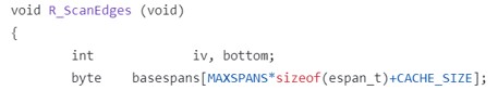
Then, once, for debugging purposes, we turned off the lighting and were very surprised to see that the graphics appeared almost flat, with the same few textures repeated over and over, as you can see in the two examples below:
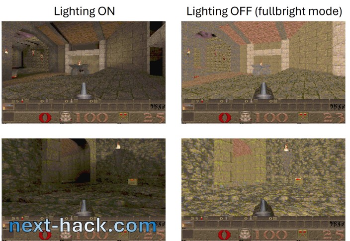
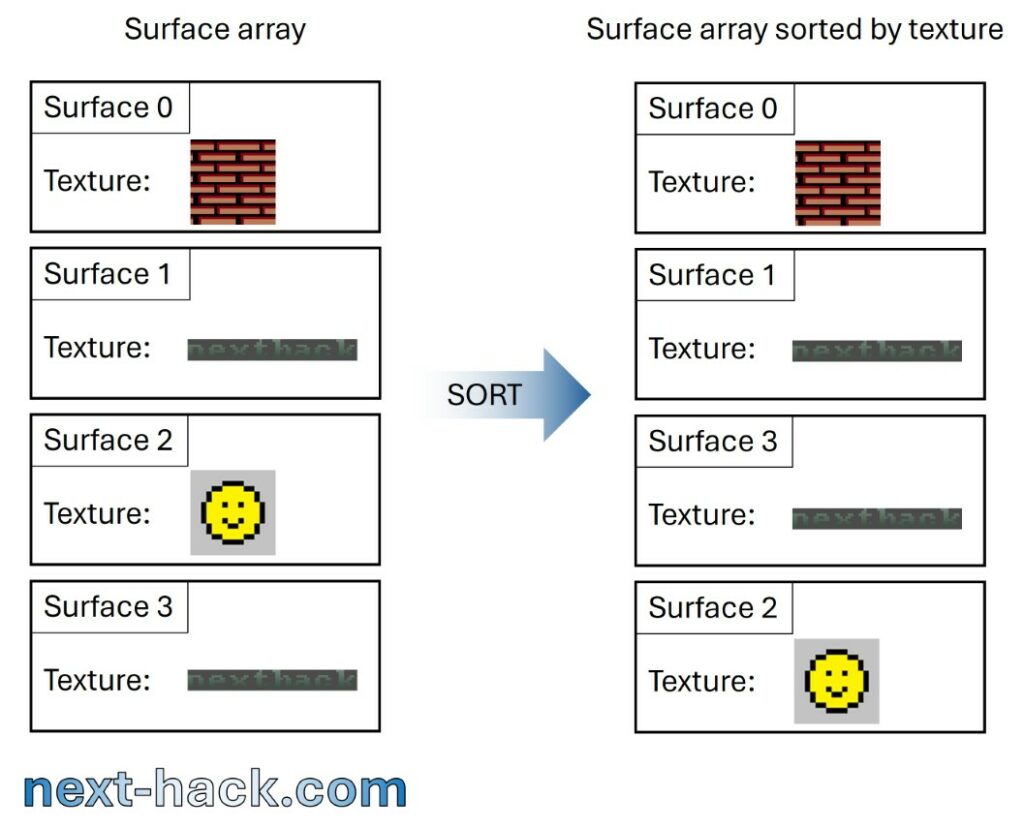
Therefore, we understood that lighting is just as important as textures in creating the sense of variety and the diverse environment that Quake has accustomed us to. This was good news, as we realized that the amount of data we needed to read from external flash for each frame could be significantly reduced. To achieve this, we needed to sort the surfaces by texture before drawing their associated spans. Sorting is done using qsort(), and its impact is minimal even in complex scenes with hundreds of surfaces; however, it significantly improves speed. Before drawing a surface, we check if the texture is already in the buffer, which saves us from an expensive load operation.
An equally important performance increase was achieved by realizing that some textures might be very small, so two of them might fit the same buffer (now reduced to about 29.6 kB, to free memory for other purposes) without increasing overall memory consumption.
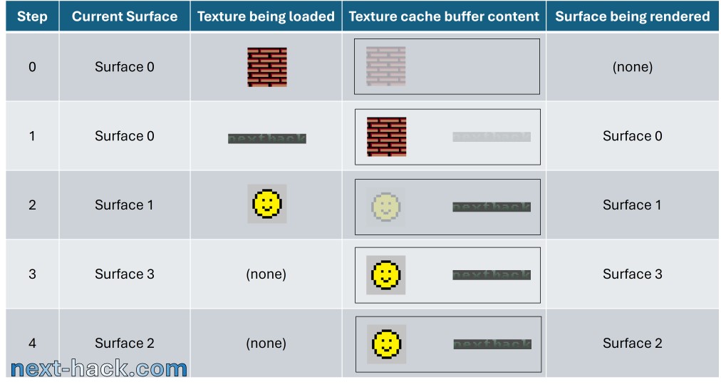
Therefore, we implemented an asynchronous load engine, using DMA, the texture cache buffer.
It works like this: let’s assume there is already a texture loaded in the buffer. If there isn’t (as may be the case when we are rendering the first sorted surface), we will simply load it and wait until it is available. Before we call the span rendering routine (which calculates per-pixel lighting using bilinear interpolation), we search through the sorted list for the next surface that has a different texture. If that texture is small enough to fit in the same buffer as the previously loaded one, we start an asynchronous DMA load. While the DMA is busy loading the texture, we proceed to render the spans associated with the current surface.
This technique is quite similar to what we implemented for Doom when drawing textures and sprites. While we render the n-th column, we load the (n+1)-th column. However, the performance increase in Quake was much more dramatic.
If the texture does not fit, we’ll simply load it after all surfaces requiring the old texture in the cache buffer have been drawn. We found that this is quite a rare event.
However, the situation is more complicated because we sometimes need to interrupt texture loading to retrieve the static lighting data of the surface from external memory as well. We encourage interested readers to examine the source code to see how this is implemented.
Moreover, the texture cache buffer would be used only when rendering surfaces, which would lead to wasted memory. Therefore, we repurpose this buffer, for instance, for:
- Edge caching: When two faces share the same edge, instead of emitting a new edge, we can reuse the existing one.
- Alias model drawing.
More details can be found in the previously shown picture when discussing memory reuse.
Optimized bilinear interpolation for surface lighting
As mentioned before, in the original code, each pixel of a surface is pre-lit, and the spans are rendered using this pre-lit image. Pre-lighting is skipped if the surface is in the cache, which greatly improves performance.
Our case is quite different.
On one hand, we typically don’t have to calculate each pixel of the rendered surface. However, on the other hand:
- We need to perform interpolation for almost all the pixels on the screen in every frame, even if we are standing still.
- We must use the full formula for interpolation, rather than simply adding a “step” value as it was done in Quake.
This process is extremely expensive, especially considering that the surface may be larger than the texture, which often has a size that is not a power of two. Consequently, for each drawn pixel, we need to perform some costly modulo operations to determine which texture pixel we should use for drawing.
There are 48,640 3D pixels, and if the above operations take 100 cycles per pixel, we would use 4.8 million CPU clock cycles per frame just for rendering the surfaces (excluding enemies, sound, etc.). This would take about 35 milliseconds for this operation alone, meaning that if all other processes take 0 cycles, our peak framerate would be just 28 frames per second on the overclocked CPU.
To improve speed, we used assembly and other strategies:
- Textures with dimensions that are both powers of two use a different routine, which employs bitfield operations to calculate the remainder. Fortunately, by profiling the demo, we found that the majority of the textures have both width and height as powers of two. As we said above, the remainder is used to determine which texture pixel should be used when rendering a surface that is larger than the texture—specifically, when the texture is tiled (repeated) onto the surface.
- For textures whose width or height is not a power of two, the remainder is calculated by exploiting integer math. A similar algorithm is used by the compiler when dividing an integer by a small constant. This process involves pre-calculating a constant through a division (which is done just once per surface) and performing two 64-bit multiplications (which are handled in a single cycle). The 32-bit version of the algorithm can be found here: https://lemire.me/blog/2019/02/08/faster-remainders-when-the-divisor-is-a-constant-beating-compilers-and-libdivide/. Since we are dealing with 16-bit numbers, the size of each operand can be divided by two.
- We extensively utilized SIMD operations. For instance, instead of separately adding the x and y values, we use a single instruction to add both.
- We leverage some FPU registers. Swapping between FPU and core registers takes 1 cycle, while loading from RAM takes 2 cycles.
- Quake used an 18×18 32-bit “blocklights” array. Each element in this array holds only a 14-bit value after the light is calculated. Using 32 bits is beneficial during calculations as it prevents overflow; however, it becomes a waste of memory afterwards. Therefore, once the array is processed, we utilize the upper half-word of each element to store the same value from the next row. This approach not only enables loading two values with a single LDR instruction but also allows for the efficient use of SIMD instructions.
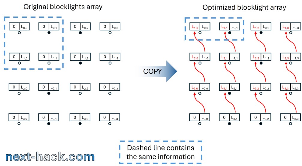
On the right the optimized one, where the same information can be loaded using just 2 32-bit words.
This also enables using DSP SIMD instructions, which can calculate on a single cycle 2 16-bit multiplications plus an addition.
- Instruction reordering. If you look at our assembly routine, you will find that it is quite hard to follow. This difficulty arises because, in the Cortex M33, many operations will take one additional cycle if you consume the result in the immediately following instruction. This is true for multiplications (including SIMD ones), floating-point operations (including VMOV, which moves data from core to FPU registers and vice versa), and so on. For this reason, we have reordered the instructions to avoid incurring the one-cycle penalty.
Originally, the C code indeed used approximately 100 cycles per pixel. The current version of the C code is even less optimized because it is designed to emulate (on a PC) what we do on the MCU in assembly, particularly with SIMD instructions, which operate on two 16-bit operands within the same 32-bit word. In contrast, the assembly code for surfaces with textures that have a width and height that are powers of two has been optimized down to about 30 cycles per pixel. The more general version, which works with textures of arbitrary sizes, is less optimized but still significantly faster than the original C code. Fortunately, such surfaces are much less frequent.
Partial screen refresh
Typically, the 3D scene changes completely with each frame, while the bottom part of the display—the status bar—changes less frequently. This occurs, for instance, when shooting (which decreases the ammo count), taking damage (which decreases both armor and health and alters color), or receiving bonuses. Issuing a full 320×200 pixel screen update, instead of a partial 320×152 update, requires more time due to three factors:
- The DMA takes 31% more time to output 200 rows instead of 152, meaning that a new frame buffer can be issued only later.”
- Since the status bar does not have a dedicated framebuffer (as it is destroyed every frame due to sharing the z-buffer memory region), it must be redrawn before issuing a fullscreen refresh. The status bar requires loading a significant amount of graphics data from external flash, and rendering it comes at a cost.
- Conversely, before rendering the surfaces in the second part of the frame (rows 75-151), we must ensure that the status bar (if needed) has already been sent, meaning the display DMA operation must be completed. Otherwise, we risk corrupting it and sending garbage to the display.
Using partial screen refreshes when the status bar does not need updating contributes significantly to increasing the frame rate. However, the first point is less important in our case, as it becomes a limiting factor only when we are operating at a frame rate very close to the hardware limit. For our scenario, the hardware limit at 136 MHz is (136/2 MHz) / (320 x 200 x 16 bits), corresponding to an extraordinarily high frame rate of 66 fps, which is never achieved, even when facing a wall.
The second and third points, in fact, are more important. Reading 48×320 pixels (excluding all the additional data for icons and numbers) from external flash takes about 1 ms when the SPI clock is set to 136/2 MHz (point 2). This 1 ms, which does not even account for the rendering time, is lost regardless of how complex the 3D scene is.
The third point becomes more problematic when simpler 3D structures are displayed, but not just when facing a wall. If the 3D view is relatively simple, it may happen that the status bar has not yet been output to the display via DMA. At 136 MHz, a full-screen update requires 15 ms, while a partial update takes about 11.4 ms. In other words, with a partial screen update, we could wait 3.6 ms less in some cases.
Remarkably, 1 ms and 3.6 ms might seem like very small values. However, gaining or losing a total of 1 ms + 3.6 ms can be quite noticeable. In fact, if we are operating at 30 ms per frame, we achieve 33 fps. Reducing this time by 4.6 ms results in a frame time of 25.4 ms, which corresponds to 39 fps. Conversely, if we add 4.6 ms, our frame rate will drop to below 30 fps.
As a final remark, you may have noticed that we recently added a new feature to our Doom port for MG24. We made this addition after discovering in Quake that the actual improvement could be significant. In Doom, in particular, we can now achieve an average frame rate of 35 fps at a resolution of 320×240 pixels, without overclocking (previously, the frame rate was limited to about 32 fps due to the maximum SPI speed). This improvement is possible because, most of the time, we only need to update 320×208 pixels via DMA. Additionally, since we are using double buffering in Doom, the first factor mentioned above becomes the limiting constraint.
Alias Models
Alias models are extremely difficult to optimize. Their texture data is stored in a rectangular bitmap, called “skin”. This skin is applied to a solid object made up of triangles.
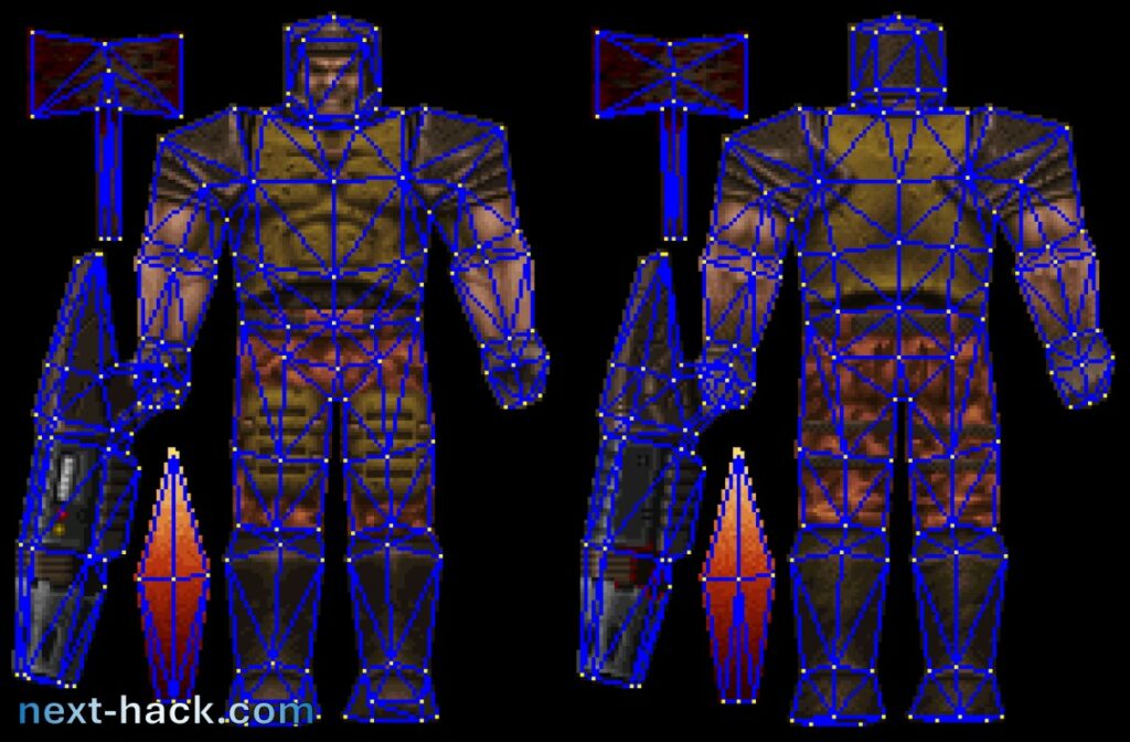
Such skins can be extremely large, exceeding 100 kB in some cases. We don’t have sufficient space to load the entire skin, so the alternatives would be:
- Issuing separate loads for each pixel.
- Identifying the square that fully contains the triangle and loading the square by rows.
- Loading (if possible) the entire skin into the texture cache buffer, if it fits (although it almost always does not).
The first option is acceptable only if very few pixels are being drawn. The second option means that, in the best case, we will always load twice as many pixels as we need. The third option is probably the most optimized for rendering, but not for loading, because it will still require loading many pixels, which may not ultimately be drawn.
There was, however, a fourth option:
- Each triangle of the skin is rasterized into columns. The pixels of each column are stored in an array, and the column arrays are stored one after another. The starting position of each column is saved in a separate array. All of this data is kept in the pak0.pak file and can be accessed from the external flash. When we want to render a triangle, we read the entire triangle data into RAM, which prevents the loading of unnecessary pixels from other triangles. The generation of the additional triangle data is performed by the utility we used to manipulate the pak0.pak file.
This solution increases the complexity of retrieving the pixel at a given (x, y) coordinate. Specifically, for a given (x, y) point on the rectangular skin, we need to subtract the leftmost x-position of the triangle from x to determine which triangle column index to use. This column index is then used to obtain the offset from the triangle offset data array, which we add to y to find the correct position in the triangle pixel data array. Despite these additional steps, this technique remains faster than a single random read or even a sequential read of the entire skin, as many pixels won’t be utilized at all. Additionally, this approach allows us to work with very small buffers, even for large skins.
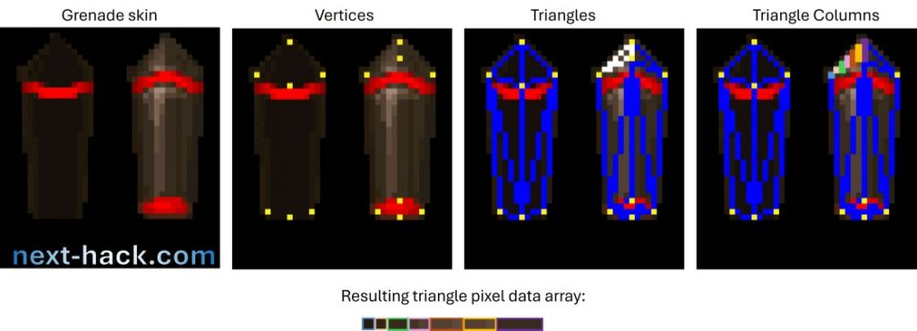
Our algorithm uses:
- Option 1, when we need to render a distant model—specifically, when the Quake engine employs recursive, pixel-based rendering for alias models—or when we detect that we will only be drawing a few pixels of a triangle for a nearby model. In these cases, random access to external memory for a few pixels is faster than sequentially reading all the pixels of the same triangle. Random pixel access is performed using the original skin bitmap, as this method is quicker for locating pixel positions.
- Option 4, when we need to draw many pixels from very close triangles (i.e., large triangles), where it is advantageous to load all the triangle pixels since many will be drawn.
Initially, we opted only for option 2, as removing the original skin would have reduced the size of pak0.pak. However, since the sky has already increased the pak0.pak size by 4 MB and we have 32 MB of external flash, we later decided to keep the original skin as well, allowing for random reads, which improves rendering by a few milliseconds.
Assembly usage
The majority of the code is written in C; however, we implemented some functions in assembly when we observed, through examining the disassembled code, that the compiler was doing a poor job. We also contacted ARM customer support to obtain a list of which 16-bit instructions are dual-issued in order to improve performance, and we used them when possible, to use one cycle less.
Additionally, we created a C-only counterpart for the assembly routines to allow us to run the code on Windows. It is important to note that this C implementation is not optimized, as it aims to emulate the functionality of the assembly code.
Global variables
Global variables are generally discouraged, especially non-static ones. The compiler compiles code by unit, which limits its ability to optimize global variables effectively. Additionally, when there are too many global variables, they may become scattered in RAM, prompting the compiler to generate a list of addresses for each global variable used in a function, placed after the function’s code. This results in slower access to global variables, as it requires reading the address of the variable from internal flash memory and then loading the actual value from that address. This process is time-consuming because there is no data cache in the flash memory, and each extra load instruction can take at least three cycles.
If access to global variables occurs very frequently (and it does), several hundred thousand cycles can be wasted just for this purpose, i.e., loading the address. We have adopted the approach that Doomhack used in his Unofficial GBA Doom port: creating a global structure that contains (almost) all the global variables. While we are uncertain whether Doomhack pursued this for speed or to profile memory usage, our goal was speed.
Notably, we did not include all the variables in this structure, as we found that doing so was sometimes counterproductive. In the end, we saved many milliseconds.
Compiler flags
The majority of the code is compiled for speed, with the exception of certain code segments that do not require optimization for speed (e.g., menus, console commands, and initialization functions), which are compiled for size. Saving flash size allows for more data to be stored in internal flash.
Selected files are compiled with the “mslow-flash-data”, to improve speed. As said before, loading the variable address is quite expensive, and this is typically put in the data section of each function, so instructions can be used instead. This increases flash usage, so we did not enable this flag for all the files, but only where we found some tangible improvement.
Math functions
Instead of sin/cos and tan we have created a function that uses precalculated values in a table. Also, usage of double has been removed, so the float-only counterpart (e.g. floorf, sqrtf, ceilf, etc.) have been used.
Too much memory optimization! Reverting back for some speed
At a certain point, we realized we had optimized too much for memory concerning internal flash. On one hand, we did not have enough flash space for anything worth storing (e.g., lightmaps), while on the other hand, we had many kilobytes that would otherwise have gone unused.
Internal flash is much faster than external flash, especially when random reads are frequent. While it is a precious resource that should not be wasted, reading unaligned data from internal flash can take many cycles, and this issue is exacerbated if we are dealing with a bitfield. We found that we could utilize some “spare” flash memory to store certain structure members more efficiently—particularly those that we had optimized too heavily (e.g., nodes and leaves). Although the structure became larger (i.e., closer to, but still smaller than, its original size), the speed increase was worthwhile. This is why you will find some preprocessor conditional directives: we tested whether specific changes produced the intended optimizations.
Another speed boost was achieved by enabling back pointers (instead of indexes) in the edge_t structure. The structure grew back to 24 bytes (the original size was 32 bytes, then it was optimized to 18 and later it was split in one of 16 bytes, plus one of 2 bytes, storing the “nextremove” index), but we gained about 1.5 milliseconds, which helped keeping up the speed in the most complex scenes. You can restore the more memory-optimized solution by setting “EDGE_POINTERS” to 0 in the file “r_shared.h”.
Noticeably, if EDGE_POINTERS is set to 1, the size of the edge data will increase. This would require to split the rendering process in two very asymmetrical steps, one of 58 lines, and one of 94 lines. This means that in complex scenes, we might get some graphical glitches due to not enough spans available. Such glitches will manifest as ghost lines at the bottom of the 3D scene. To counteract this, if EDGE_POINTERS is set to 1, we reduce the number of edges from 1800 to 1600 (so that the two rendering steps are 65 and 87) , and we increase the number of spans to 3650. feel free to set EDGE_POINTERS back to 0. It is worth noting that the figures about memory occupation/reuse are shown for EDGE_POINTERS 0.
External C-Tools
We developed several tools for this project.
- The aforementioned pak0.pak file converter (MCUPackConverter). This program:
- Pre-calculates all the sky images
- Resamples all sounds to 11025 Hz, mono, 8 bits.
- Creates the triangle data for the Alias models.
- Handles brush models (including level world model) so that these can be used more efficiently from memory or speed viewpoint.
- Output a list of all the strings found in the PAK files, to be included in the code in pakStrings.h
- QTablesGenerator: creates constant tables used for instance for math functions.
- QuakeCConverter: takes all the “.qc” script files and generates the C code.
- FunctionArrayGenerator: generates all the setters and getters, and the arrays containing them, for all the class of edicts.
All the tools above neither change the behavior, nor reduce the graphics details/map complexity of the shareware Quake.
Our port In Action!
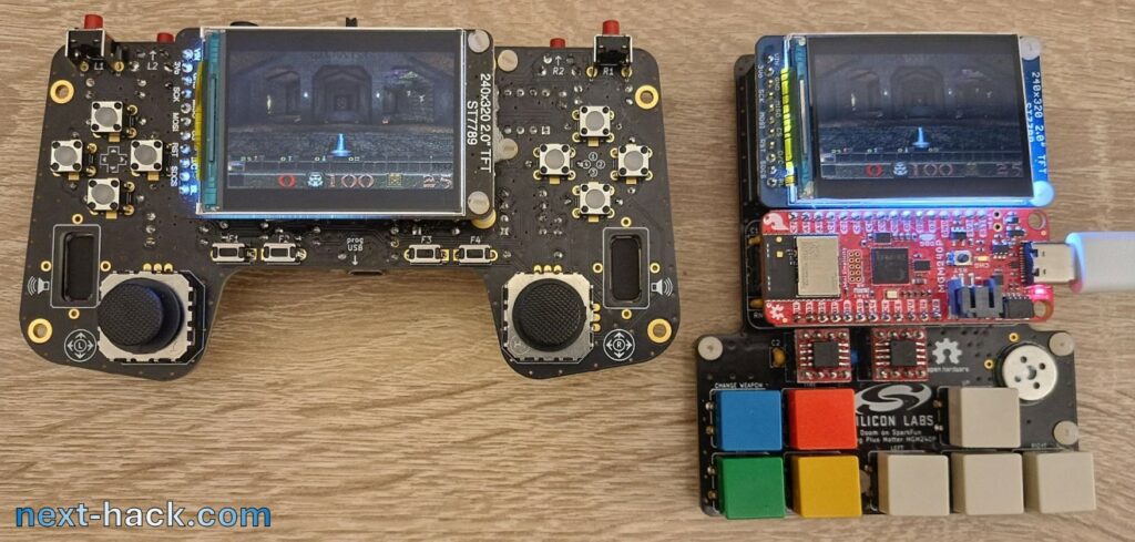
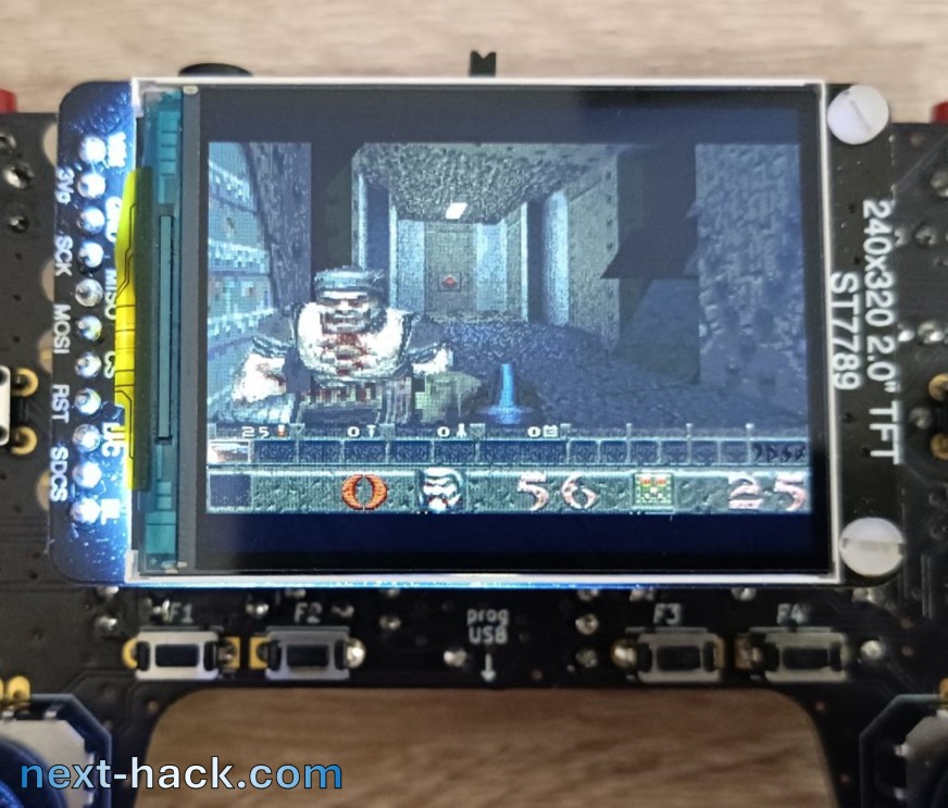

You can see more pictures at the end of the article.
Want some video? Here it is!
Speed and Comparison with Other Ports
2024/11/02 Update: this section does not reflect current version 2 performance, which has improved! See the new article for more information.
As we said before, the initial speed was very slow, and during the demo playback, the frame rate initially was between 7 and 10 fps, with overclocking.
After all the optimizations cited above, we were able to increase the speed noticeably. The frame rate of the timedemo of shareware demo3 now ranges between 17.7 and 45.6 fps, averaging at 28.0 fps in demo 3, with overclock. Without overclock, the figures are divided by a factor 1.7: between 10.4 and 26.9 fps. In the plot below we show, the time required to render each frame of such timedemo. We also show the more interesting reciprocal value, the instantaneous frame rate. The framerate varies quite a lot, but very rarely goes below 20 fps.
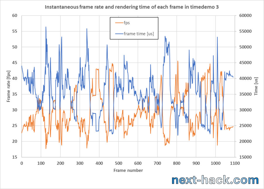
Note: in our code, we print to the USB Virtual COM the time taken for each frame (including not only the 3D rendering, but exactly how much time (in microseconds) has passed since last frame, i.e. including game logic, physics, etc.). You can use Teraterm or other software to get such data. To determine the frame rate you must simply divide 1 million by that time. E.g. if you get 25000, then the instantaneous frame rate is 40 fps. You can also use the cheat code in the console “showfps 1” to enable the instantaneous framerate to be shown in the bottom left corner of the 3D viewport.
The first map (E1M1) has an initial framerate of 26.3-27.5 fps and during the whole gameplay is very enjoyable. The actual in-game instantaneous and average framerate depends on many factors, such as scene complexity, number of on-screen objects, number of particles and even number of active sound channels. This mostly derives from relatively slow external flash accesses.
For instance we have seen instantaneous frame rate values as low as 15 fps and higher than 45 fps. Still the fact that a single frame took 66 ms, does not mean that the frame rate is really 15 fps: it would be 15 fps if, for a consistent amount of time (e.g. 1 second), all the frames required 66 ms on average. We found that typically this is not the case. Vice-versa, when the instantaneous time to render a frame is 20 ms, does not mean that the frame rate is 50 fps: it would be 50 fps if many frames (e.g. 50) took 20 ms on average. Still plotting the instantaneous frame rate is a good tool to identify performance bottlenecks.
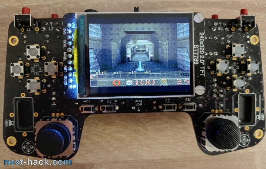
You can watch the frame rate in the video embedded above.
How does this compare with other ports?
To our knowledge, beside many PC ports, there are very few ports to microcontrollers.
One is a port to the STM32F747 microcontroller and another is a port to a dual core RISC-V MCU. The source codes of these ports are basically the same as WinQuake: the only modifications are on the hardware abstraction layer, to run Quake on the target board. These MCUs are very powerful (480 MHz superscalar Cortex M7, and a dual-core 400 MHz RISC-V), and both boards they are mounted in have at least 8MB RAM. These specs are enough to run the stock Quake, so no optimization effort was spent in terms of memory and speed. Indeed, we see from the videos that Quake runs very fast on them, and, in particular, from this video, we see that the framerate is between 30 and 75 fps. This is not surprising, as we expect that a 400 MHz RISC-V is between 2.5-3 times faster than a 136 MHz Cortex M33. A 480 MHz Cortex M7 is also more than 5 times faster than a 136 MHz Cortex M33 (taking into account that the CM33 has 1.5 DMIPS/MHz, while a CM7 has at least 2.3 DMIPS/MHz).
Noticeably, on per MHz basis, we run at similar or even higher frame rate/MHz, with respect to the previously mentioned ports. This is happening, despite we must fetch the majority of data from the relatively slow external flash, instead of RAM, and despite we don’t have the surface cache. We think this is both surprising and remarkable.
Instead, Randy Linden’s port to the GBA runs slower, but only because the system is much less powerful than ours. Yes, the GBA port renders only one-third of the number of 3D pixels compared to ours. In fact, not including the status bar and taking into account that the horizontal resolution is halved, Randy’s port has 120 x (160 – 24) = 16,320 pixels, while we have 320 x (200 – 48) = 48,640 pixels. Additionally, the initial framerate on E1M1 is 9.5 fps on the GBA, while it is 26.3-27.5 fps on our system.
However, if we consider that our 136-MHz Cortex M33 (1.5 DMIPS/MHz) has an integer performance 13.3 times that of the 16.7 MHz ARM7TDMI (0.9 DMIPS/MHz), on a rendered pixels-per-second-per-MHz basis, Randy’s port is actually 60% faster (i.e., x 1.6) than our port. This is likely an underestimation of how optimized the GBA port was, because our MCU has a built-in FPU, while the GBA port had to rely solely on integer math.
Still, there are some differences between the two ports:
- Our port uses assembly only for few functions, while, according to the article cited at the beginning, the GBA port uses about 200k lines of assembly.
- The GBA display resolution requires a frame buffer of only 38400 bytes (note: in this case we must consider the full display resolution, and not only the 3D pixels). The z-buffer, instead, requires a number of bytes which is twice the number of 3D pixels: 30 kB. Instead, in our case, we are using 142.5 kB (for frame + z buffers). The GBA also has 384 kB while we have 276 kB.
- The GBA has a fully memory-mapped cartridge with a parallel interface. According to this site, the cartridge can be accessed with 0 wait states. Since the bus width is 16 bits, the peak bandwidth is 33.4 MB/s. The latency is 2 CPU cycles (for a single LDR instruction), which equates to 120 ns. This performance is much worse than our internal flash, which has a bandwidth of about 181 MB/s and a latency of around 20 ns. However, the internal flash is much smaller and cannot contain everything. In contrast, the external flash has a peak bandwidth of 17 MB/s (roughly half that of the cartridge) and a latency of a few microseconds. From a constant data access perspective, this means that the GBA may be quicker.
- The GBA port does not implement the whole game logic, enemy AI, and level switching. For instance, as reported in the article, enemies react only when you shoot at them, and level must be switched manually. From the video, one understands that end-level teleports do not work.
- We are not sure if the sound is implemented in the GBA Quake port. Sound not only has some marginal impact on speed but also affects RAM usage.
- We kept all the features such as demo, console and cheats as well, while it seems to use that these are missing on the GBA port.
- Save games are fully supported in our port.
- By analyzing the images on the video, we understand that (at least in the Quake port) bilinear interpolation for lighting is missing: light varies abruptly between what seems to be 16-pixel square. This was later implemented in the derivative work Cyboid, by Randy.
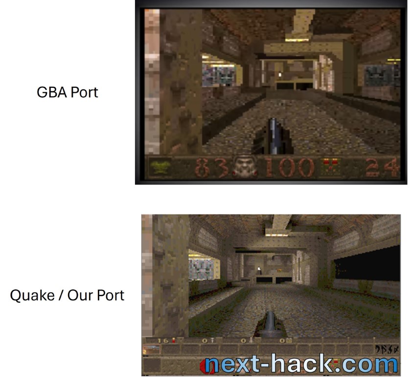
What about the comparison against Quake running on a PC? We used the data reported in this site to make our comparison, and we ran the same timedemo, with the same settings. We achieved 28.0 fps, with our overclocked system. This is more than 1 fps faster than a Pentium 100 running at the same resolution, and still a bit faster than a 6x86MX PR200 (27.4 fps).
In those systems reported above, however:
- Quake had a lot of assembly-optimized code.
- Surface cache was available.
- Data was stored in RAM, and was not read from external flash, which has rather limited performance in our system.
Also, our benchmark is taken with audio, whereas data reported in the previously cited site is without (-nosound option).
Build your own!
Hardware
We don’t sell hardware or software. We provided the design files in the Github repositories linked in this article, so you can easily build your own and, why not, improve it!
If you have a Sparkfun Thing Plus Matter board, you can use the same hardware we developed for previous Doom project, with two exceptions:
- The gain-setting resistors of the audio section should be changed because of the different sound configuration, as explained previously. If you don’t make this change, the audio will be very quiet. To overcome this, R4 must be now between 68-82 kOhm, and C15 must be decreased to 68-82 pF, see schematics.
- You must use 16-MB Flash ICs, not just 8-MB ones.
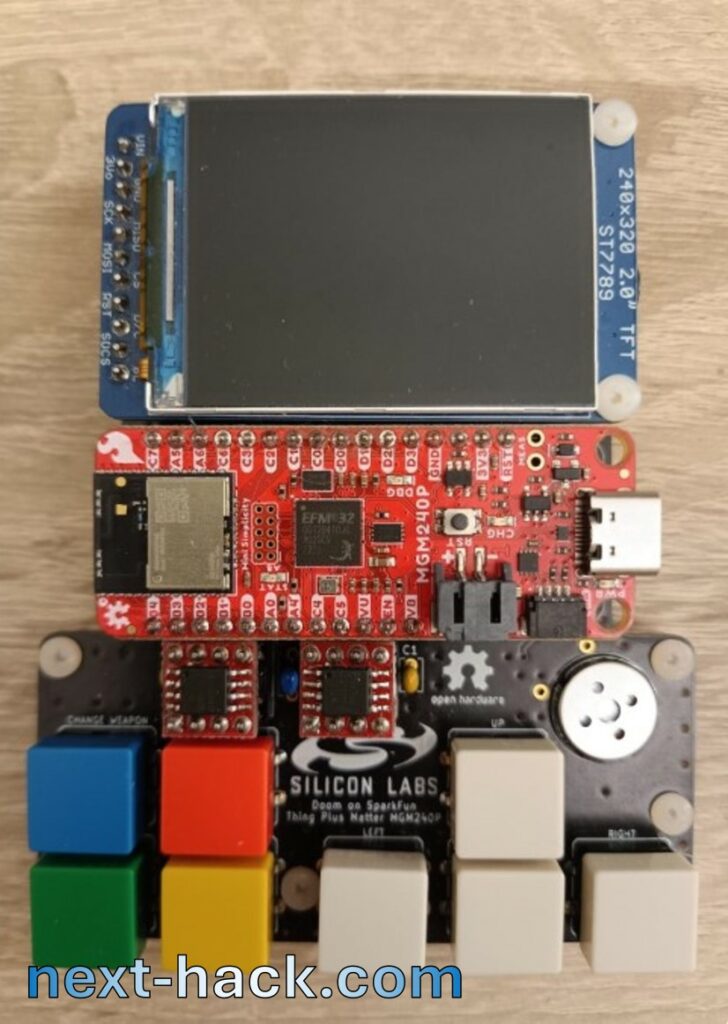
Instead, if you have an Arduino Matter Board, you can build the new PCB, which has more buttons, built-in stereo audio, and two analog Joysticks. Soldering the complete kit is a matter of 1-3 hours, depending on your skills. The KiCAD schematics and PCB layout file are of course available on the Github repository.
Firmware
Download the MG24Quake repo and unzip it somewhere (e.g. C:\MyDir\). Then open Simplicity Studio 5 (yes, we assume you have downloaded it!). Make sure you have the Gecko SDK 4.4.3. If you don’t have it, in Simplicity Studio, choose Update Software from the Help menu and find in the GSDK 4.4.3 there.
Then, select “Import…” from the file menu. A window will appear. Click on “browse” and navigate to the QuakeMG24 directory, in the dialog. You should see these two options: select the second one (i.e. with .sls extension).
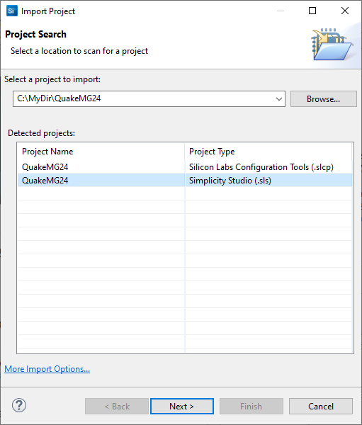
Note: we had not too much time to clean up the code, which is, at the moment of writing, full of dead code, and things that shall be simply deleted, which were used for profiling, testing, debugging, troubleshooting. Also, we used the same code to develop/test in Windows, so you’ll see many conditional defines that check if we are compiling for Windows (#if WIN32).
SDK File Generation (mandatory!)
We are licensing all of our code in LGPL, which has the side effect that we cannot include Silicon Labs’ Gecko SDK (still freely available after installing Simplicity Studio, a free IDE by Silicon Labs). The project must be imported and, and “regenerated”. Project regeneration will reinstall into the project the missing GSDK folder.
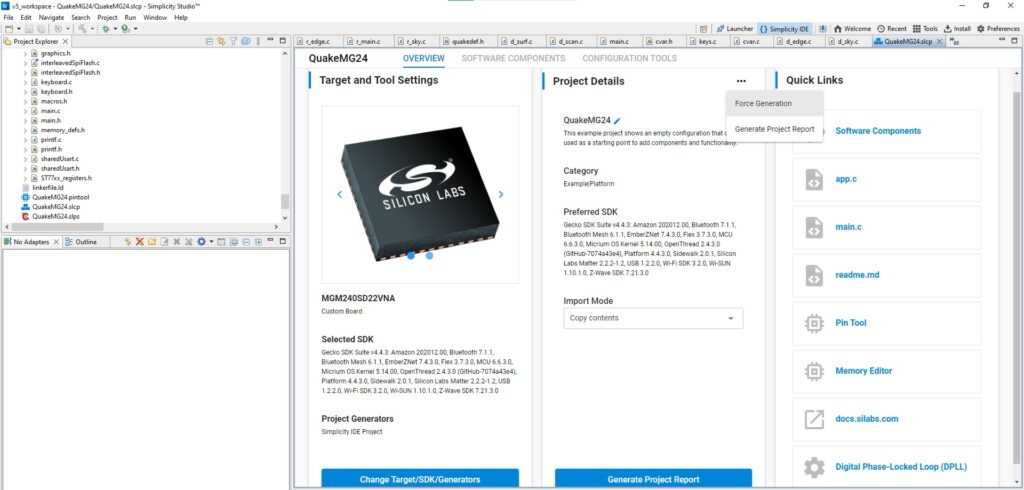
We are using Gecko SDK 4.4.3. This is not the latest SDK (now called Simplicity SDK), because when the project was started, the new SDK was not available. Make sure you have this SDK version. If not, you select “Update Software” from the “Help” menu, and then download the GSDK 4.4.3
Building
There are two build configurations. One is for the old console (build configuration “SparkDoom”) and the other is “TheGamepad (Arduino Nano Matter)”. It should compile without warnings.
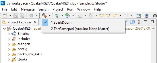
Note: as stated above, we leave on by default the demo sequence. This will wear the flash out, if you leave it running for about 7 days! We strongly recommend to disable demo by changing the ENABLE_DEMO definition in Quake/quakedef.h to 0.
Flashing
Connect your board to the PC USB, and follow one of the two procedures below.
Note: if you are using “The Gamepad” then you must use the debug USB connector (i.e. the one of the Arduino Nano Matter board) and NOT the battery charger module connector!
Using Simplicity Studio (Sparkfun Thing Plus Matter Board only)
At the moment of writing, Simplicity studio can be used to compile the firmware, but it will be able to flash only to the Sparkfun Thing Plus Matter Board.
To do this, you must right click on binary and then “flash to device”, and finally, click on the “flash” button in the windows that will open.
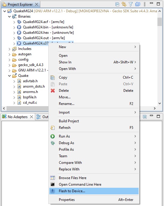
Using bat file in /TheGamepad (Arduino Nano Matter)/ subfolder (Arduino Matter Board only)
To be able to flash to the Arduino Nano Matter board, you must have installed the Arduino 2.x IDE, and in the IDE, you should add the support package for the Arduino Nano Matter Board. This will install the required programming tools. You might find a more detailed description in this article.
To program the Arduino board, you must find the file “CopyToArduinoMatterBoard.bat” in the subdirectory “TheGamepad (Arduino Nano Matter)”, and execute it. This will use openOCD (installed by the Arduino Nano Matter board package) to upload the image to the Arduino Nano Matter board.
Pak Conversion and Upload
First of all, you need the shareware pak0.pak file. Note, this is the only version, that it is supported. You can find it by googling “Quake shareware”.
However, before you can upload it to the device, you MUST convert it, using our MCUPackConverter Utility, you can find on the repo. You might choose to recompile it (we used Code::blocks), or you might find the executable in the “MCUPackConverter\bin\Debug” folder.
The utility can work in two ways: with or without parameters.
- Without parameters. This is the fastest way. You have to put executable in the same directory where the pak0.pak file is, double click on the MCUPackConverter.exe. Press any key when asked, and after the program finishes, the pak0conv.pak will appear in the same directory. Note, the converter will vomit a lot of strings, you can ignore!
- With parameter.
Open a command prompt and enter:
MCUPackConverter <input file> <output file>
After you have the converted pak file, rename it to pak0.pak and put to a microSD card. Then
- Insert the micro SD card to the device you want to install the pak0.pak to.
- Power on the device you which to program, and keep pressed the buttons UP, DOWN and ALT and FIRE at the same time if you are using the Sparkfun Thing Plus Matter board. If you are using “The Gamepad” you must press up-down and the buttons 3-4 on the right side.
- The program will automatically erase the external flash (this will take up to 100 seconds) and copy the file from the micro SD card to the external flash (this will take about 100 seconds as well). Note: unlike our Doom port, we don’t support Y-Modem upload anymore. That’s terribly slow (about 50 times).
After you flashed the pak0.pak, we suggest you to remove the SD card, because we found that at high speed, it might create some glitches on the display.
Some more pictures
You can see below: console, cheat (we show it by getting all weapons in the start map), control, some levels with frame rate (including secret level!), underwater warping, savegame, etc.
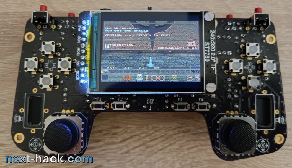
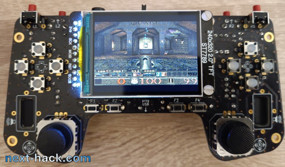
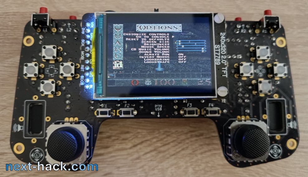
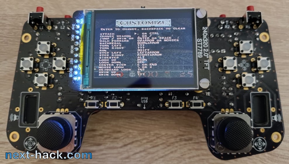
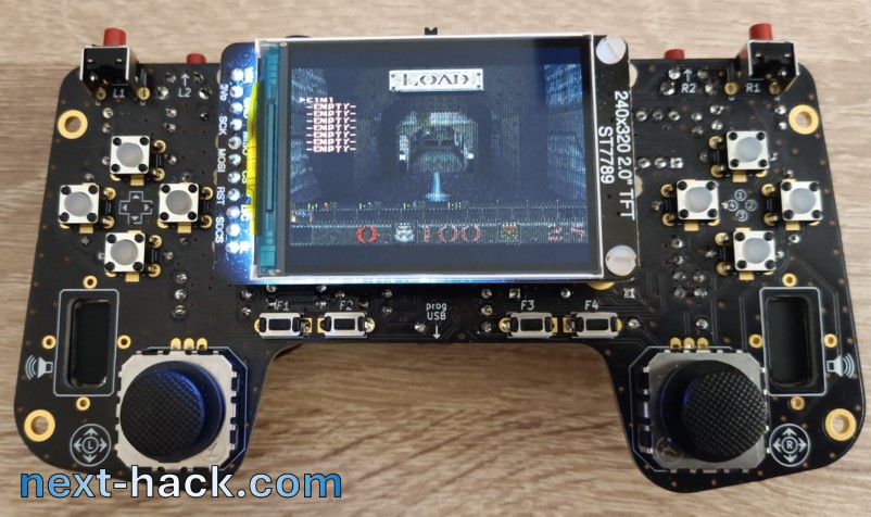
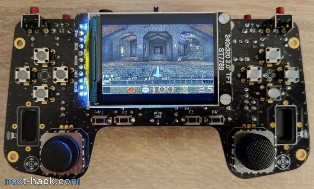
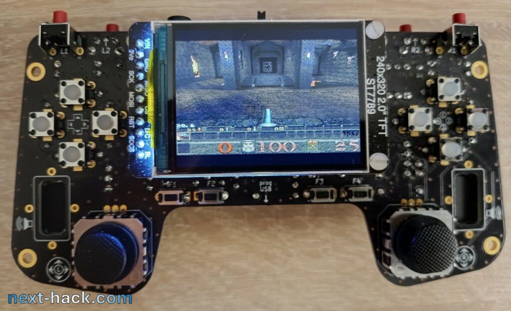
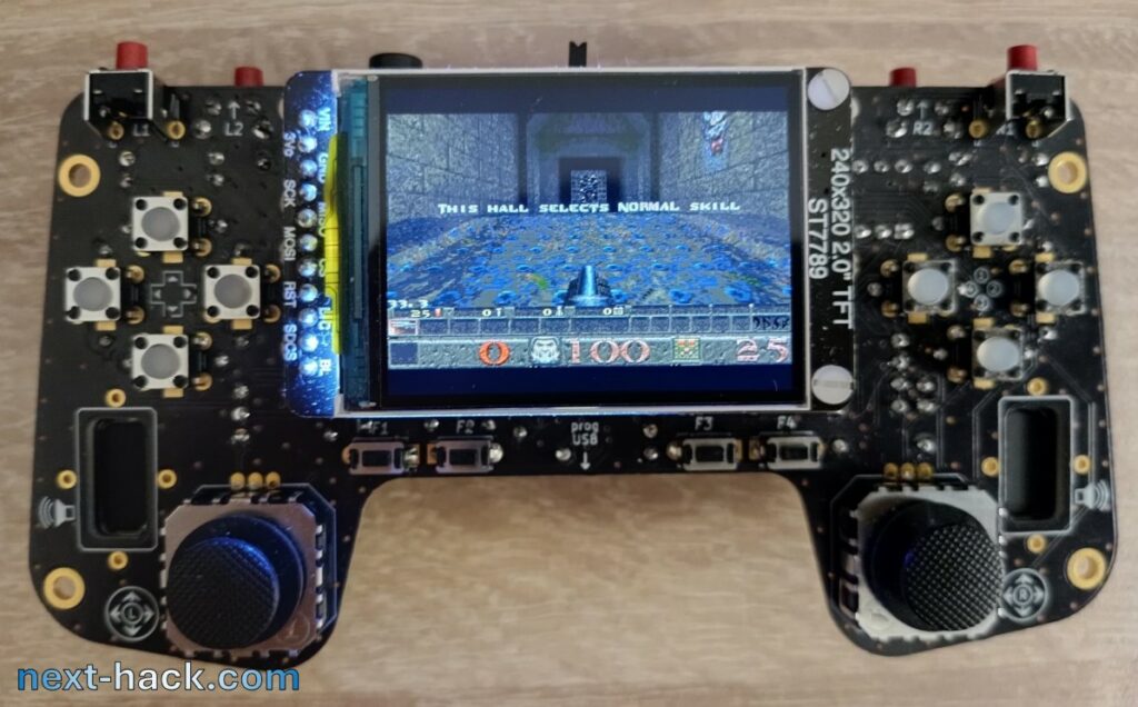
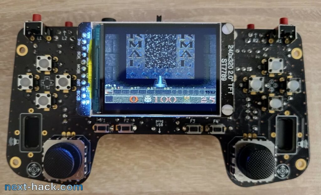
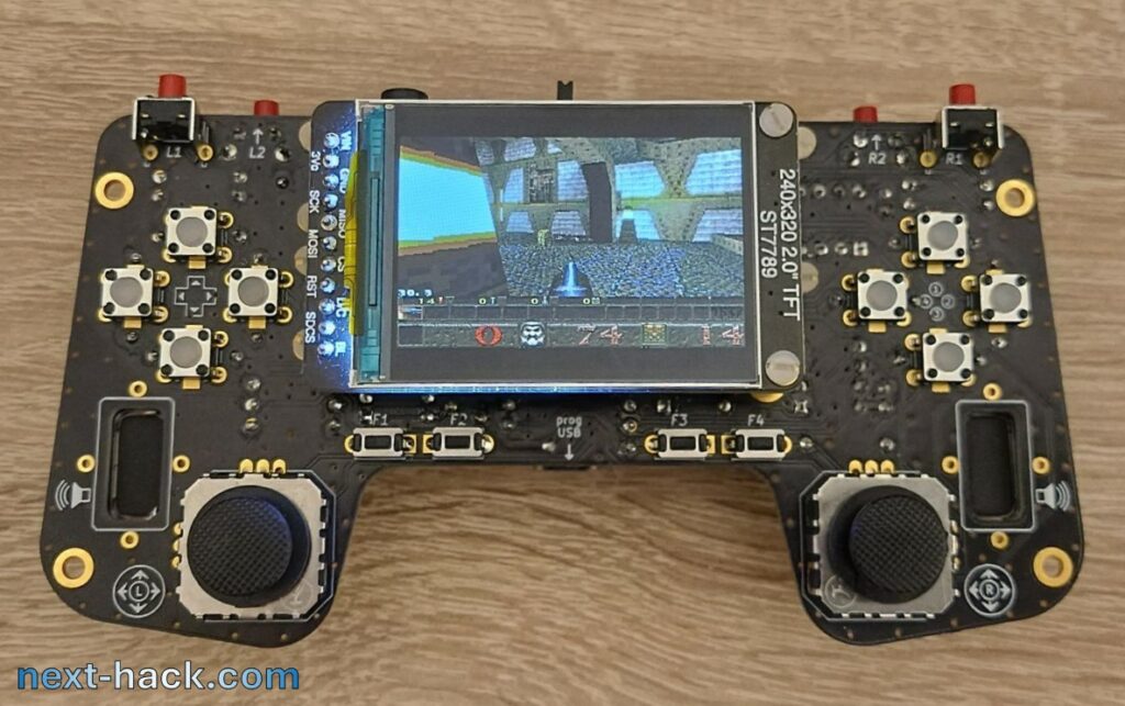
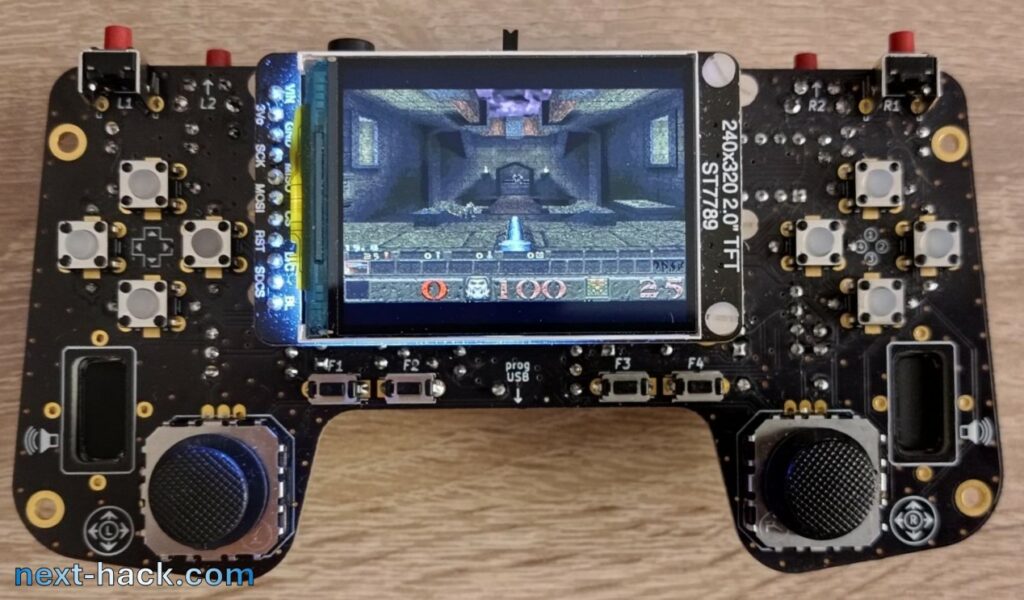
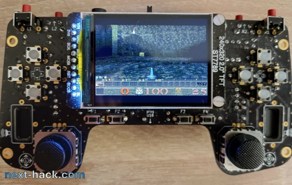
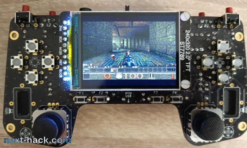
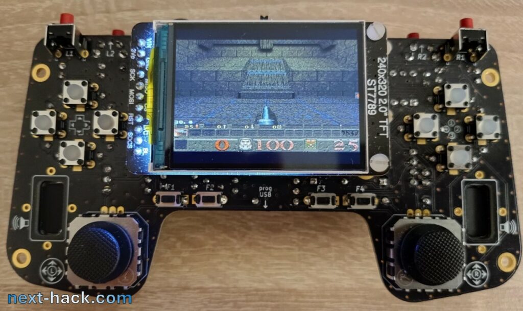
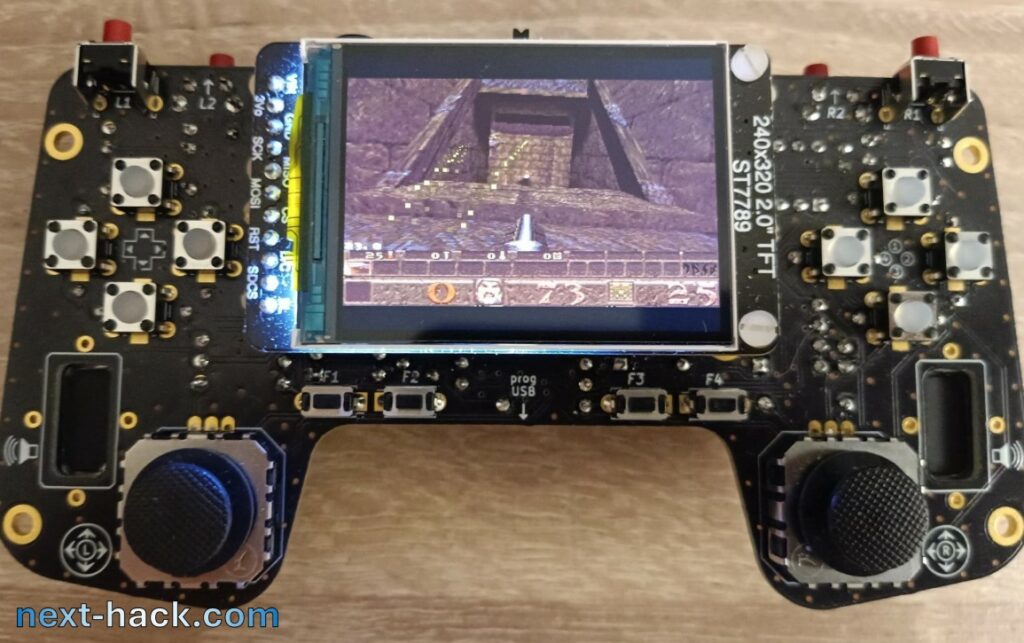
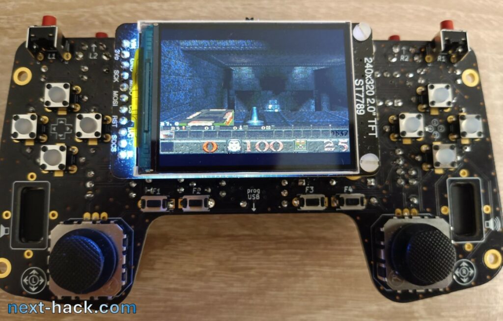
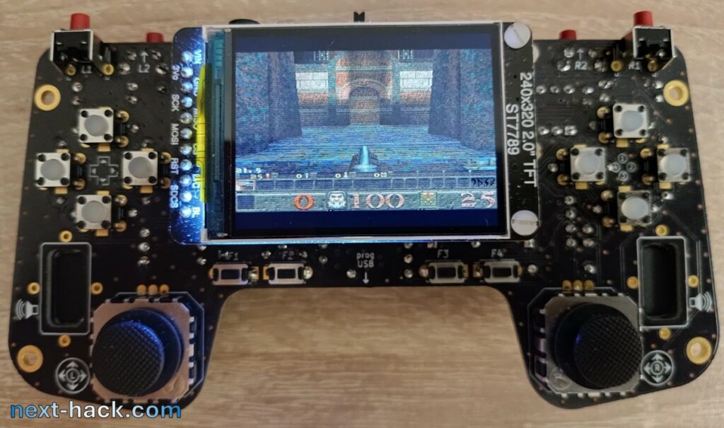
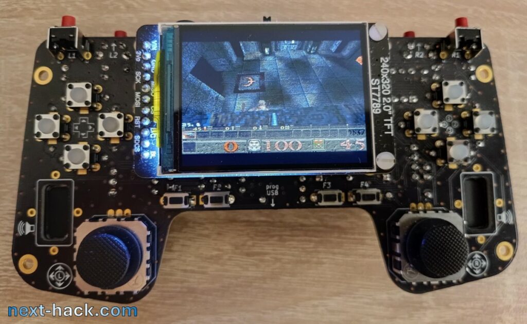
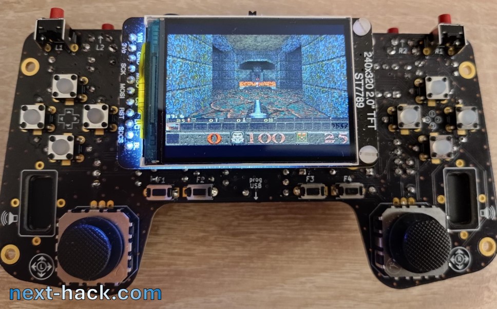
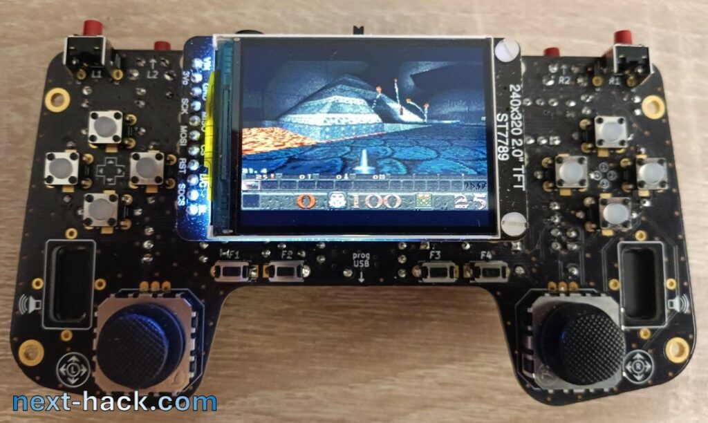
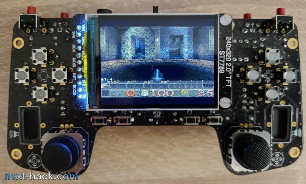
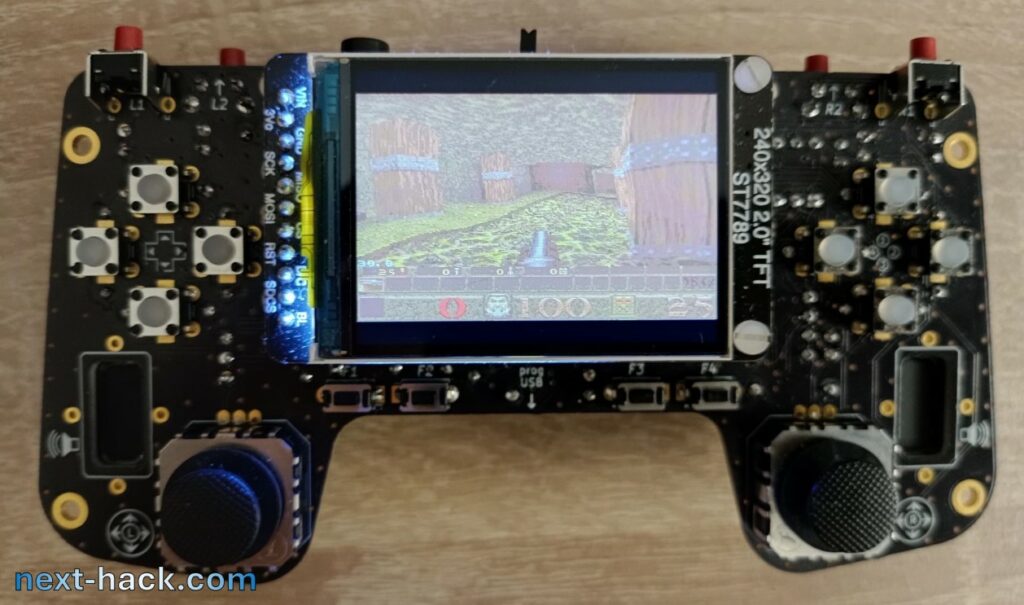
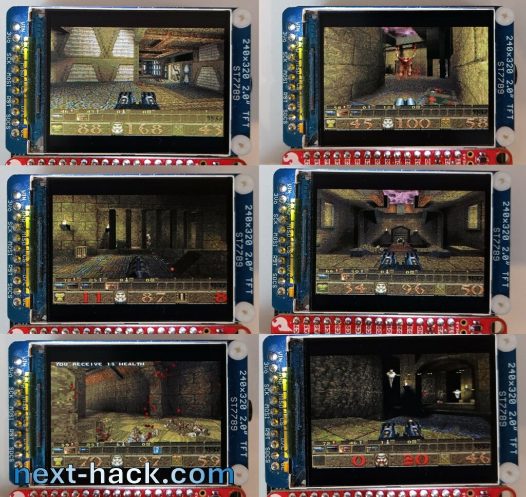
Conclusions
We admit this was the biggest and most difficult project we worked on so far. It took many weekends, holidays, and even nights of hard optimization, especially on the memory side. The port required us to create four additional tools, modifying completely some drawing algorithms, and probably changing some thousands of lines of code.
Still, not only all the mandatory goals of our challenge were met, but also all the features were implemented in this port, including the “nice to have” ones (such as savegames, settings, cheats and console). We only left out music and multiplayer, the former due to lack of CD player, the latter because of lack of memory. We also left out screen resizing and of course resolution change: it is fixed to 320 x 200, with standard 48-pixel tall status bar.
Level switching takes 12-13 seconds, and we think that we could improve this figure by some seconds, but this was outside the scope of the work. Reloading a savegame from the same level (with same difficulty level) takes less than one second.
Very surprisingly, on per MHz basis, the speed of our port is comparable to what it was achieved using the stock WinQuake codebase on other MCU based systems, despite they had much more memory (at least 8MB), and they had not to load everything from a relatively slow external flash.
Still, we think that speed can be improved even more, especially if assembly is going to be used more extensively. To get more substantial increases, probably some algorithms should be completely changed.
We also believe that there is still room for more memory optimization, but for Multiplayer implementation a completely different approach will have to be taken.
We estimate that, in systems with few tens kB more (e.g. 64-128kB), the multiplayer experience could be very easily added, and probably a speed boost is also expected. With such RAM increase, we could restore also the support for the retail Quake PAK support, provided that enough external flash is installed. This will require also to support 32-bit SPI flash IC addressing. (2024/11/02 edit: we managed to run the full retail game without requiring more RAM!).
Yes, there are many microcontrollers that feature more RAM and/or internal flash. Without looking too far, for instance, the EFR32MG26 has 512 kB RAM and 3 MB internal flash, and the same core speed. With that MCU for sure we could implement the multiplayer and have a noticeable speed boost. However, at this point, this would be much less of a challenge, if any at all.
See you soon for our next hack!
Acknowledgements
We would like to thank:
- Id Software for making Quake and releasing its sources.
- The owner of this youtube channel for the very clear and mind opening explanations about the Quake engine.
- The owner(s) and contributors to QuakeWiki, for the very useful information that can be found there.
- Modern Vintage Gamer for the video about Quake being ported to the GBA. This was what started this project.
- The owner(s) of https://thandor.net/, for the very useful benchmarks.
Downloads
- The Gamepad design files: https://github.com/next-hack/TheGamepadDesignFiles
- MG24Quake and Tools full source: https://github.com/next-hack/MG24Quake
Appendix A – Timedemo
If you are familiar with Doom and Quake, you probably already know what a timedemo is.
Before we look at the timedemo, let’s briefly explain what a demo is. A demo is a recording of a game. It contains enough data for the engine to reconstruct the match that was played with 100% fidelity. Doom and Quake, as previously mentioned, have different strategies, but the result does not change; when you play it back, you will get the same outcome regardless of the machine you are using, from a match viewpoint: duration, rooms visited, enemies killed, damage taken, shots fired, etc. What changes is the number of frames that will actually be rendered. In fact, a slow machine will take a long time to render complex frames, so the demo playback engine will skip rendering some frames to match the real game speed. In Quake, if your device is very fast, additional interpolated frames will be rendered for smoother playback. In Doom, if your device is very fast, the framerate will cap at 35 fps, and to achieve this, a variable delay will be introduced.
Instead, in a timedemo, we render all the stored frames (note that the frames themselves are not stored. In Doom, we only store the player’s keyboard input, while in Quake, we store the entity data, such as frame, position, angles, etc.). There is no frame skipping, intermediate frame calculation, and no delay is added between frames. In this way, every device, regardless of its computing power, must render exactly the same scenes, which can be used for a “fair” comparison.
If a system is extremely powerful, the timedemo will run very fast, and will take a very short time, much smaller than the time the match took when it was recorded. Conversely, slower machine will take longer time. This total time is used to calculate an average framerate: each demo stores a fixed amount of frames (e.g. 1000 frames), so to get the average framerate one has simply to divide this number by the time it took playing it back at the fastest possible speed.
For instance, if a demo has 1000 frames stored in it, and it takes 40 seconds for its playback, the frame rate is 25 fps.
Measuring the time it takes to render the same set of frames is a far better benchmark than simply counting the frames rendered during a regular demo playback. In fact, skipping or interpolating frames can lead to a different subsequent frame, which may take more or less time to render, resulting in an unfair comparison. For example, consider a demo with 1,000 frames recorded at 20 fps. It should last 50 seconds. Suppose that the first 20 frames are very complex and take your machine 1 second to render, while the next 980 frames are rendered at exactly 20 fps. In a regular demo, you would render 981 frames in 50 seconds, achieving an average frame rate of 19.62 fps. However, with a timedemo, you would render all 1,000 frames, but it would take 980/20 + 20 = 69 seconds, yielding an average frame rate of 14.49 fps.
Notes
[1] According to IGN and Gamespot.
[2] The internal flash is one order of magnitude faster than external flash for sequential reads. This speed difference increases to 2 orders of magnitude in case of random reads.
[3] Actually we put a 10kOhm input resistor, which means that the gain is only 8. If you prefer using DAC, you can change this value to, say, 330 Ohm or lower, and get back to the gain of 16, using the DAC.
[4] For a better understanding how rendering works in Quake, you might look at these very interesting videos: https://www.youtube.com/watch?v=IfCRHSIg6zo and https://www.youtube.com/watch?v=zdXsHWHxeBY
Hi, when you write “while the 64 bit bus allowed for 240-320 MB/s peak bandwidth (tPC = 33 ns and 25ns, respectively).”, you are grossly overestimating the actual 1996 era memory bandwidth, as reported by user rasz in https://news.ycombinator.com/item?id=41711371#41736631, who points out that the expected BW will be between 50 and 70 MB/s. Although this is still larger than 17MB/s, these are not 20 times slower but 3.
Hi Smiru,
thank you for the valuable information. We agree, our was a really crude overestimation. We also checked some benchmarks on the net, and the reported figure 50-70 MB is also in the range of what other users have shown in their benchmarks using different programs.
Still, these figures are better than the 17 MB/s we can hope for at the best case. At the worst case we go much slower, especially for small transfers (e.g. 8 bytes).
We have changed the text accordingly.
Thank you again!
Hi, Not sure if the previous comment was blocked by antispam because of the link, could you please check the the questions about peak bandwidth of 1996 era PCs being overestimated?
Hi again!
see answer to your previous comment!
Hi I just wanted to say congrats on your work! I’m the guy who did STM32 port while back. Yes it was very limited work mostly just HAL port. My goal was to push even further to some Arduino boards but then my life was getting busier and gave up 🙂