
Introduction
Hi there!
In the previous episode we showed you how to enable 8MHz transfers on the popular 1.8” Display+SD shield. If you didn’t read it, go and check it, because it will be required for this episode!!!
In this episode we want to address another issue: is the SPI module of Arduino’s ATMEGA328 fast enough for our devices?
This question is legit, in fact, if you consider the time taken by the test program (either with a scope, or by using the “Serial Monitor” function on the Arduino IDE), you’ll notice that there is something going wrong: if the SPI is clocked ad 8MHz, you would expect 1MB/s, therefore you should read your 900kiB (924kB) test.bmp file in 0.9s, whereas it takes about 2.4s., i.e. only 375kB/s.
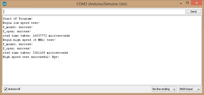
Fig. 1: Serial output from the SD card test code of the previous episode.
Note: in this article we consider M = 1 million and k = 1000. ki denotes 1024 and Mi denotes 1048576, i.e. 1024 ki. For sake of simplicity, in the video we don’t make this distinction.
This is well below the expected 1MB/s! Less than 40% of the theoretical throughput!
Of course, there is some software overhead (due to the FATfs library), and when the file pointer crosses the cluster boundary, the Fatfs needs to read the FAT table, in order to know the sector at which the next cluster begins. Also, there is a transmission overhead, because we must send – through the same SPI lines – several bytes composing the command to actually ask the SD to read one or more sectors. Finally, when we send a low-level read command to the SD card, it will take some time before data become available. This time depends on the SD card and on the type of read command: read single or read multiple blocks. If we just read a single block (as in our case), this delay time might be a substantial fraction of the total time taken by the actual read-out. In our case, we verified that the card takes over 225 microsencods! That’s a huge amount of time! These non-SPI related overheads are explained in the video linked at the bottom of the page.
So, to read the 900kiB of file, we need to read 1800 512-Bytes sectors. That means that 225*1800 microseconds are wasted, i.e. more than 0.4 seconds (note: reading in chunks larger that a single sector will for sure reduce the total time we are waiting). Therefore the time taken to read the actual data is about 2 seconds, i.e. we read at 450kB/s.
This again includes some software overhead, the time taken to send the SD command and the FAT readout. Still, we are less than half of the bandwidth one could expect from a 8MHz SPI. Is this due to software-only overhead, or is it due to the SPI module, being somewhat inefficient?
We will find out that the SPI plays a major role.
In fact, the SPI has single buffered writes, that is, the transmit register (SPDR) is also actually the transmit shift register, therefore you can’t write a new byte, while the SPI module is still sending the old one.
In order to see if you can send new data, you must check if the SPIF bit of the SPI status register (SPSR) is set to one. In other words, you must use the following instruction in C:
loop_until_bit_is_set(SPSR,SPIF);
Which translates into the following assembly instructions:
Wait_Transmit: in r16, SPSR; (Load SPSR to register r16)
sbrs r16, SPIF; (SPIF bit set? exit)
rjmp Wait_Transmit; (jump to the first instruction)
(Note: We used r16 as example. The actual register number used will depend on your program. The particular register used will not affect the timings).
The first instruction (in r16,SPSR) takes 1 clock cycle. The second one takes 1 clock cycle if the bit was not set, otherwise, 2 clock cycles. The third one takes 2 clock cycles.
As you can see, in the best case condition, you must wait 3 clock cycles before you can send another data (only the first two instructions would be executed), which will start the one cycle later.
Therefore you waste at least 4 CPU clock cycles when sending one byte, which is 16 cpu clock cycles long. I.e. at the best case, you need 20 cpu clock cycles to transmit 8 bits. In other words, instead of sending at 1MBps you’re sending at only 0.8 MBps. This is not even close to what we reached in our example.
Still, to save those 4 lost CPU cycles, one might be tempted in writing the following trivial code:
Write data to SPDR.

Wait Exactly the minimum number of cycles required for the transfer to complete.

Write again new data to SPDR.
If you wanted to transmit data at the full sustained 8Mbps data rate, you should wait 15 CPU cycles between two consecutive writes to SPDR, so that for each byte you have 15 wait cycles + 1 write cycle (OUT instruction). In other words, 16 CPU cycles that is 1 us every 8 bit (i.e. 8Mbps or 1MBps. Please note that 1MBps = 1Mbps, as the B stands for byte and b stands for bit).
You’ll find that 15 wait cycles are not enough: if you only waited 15 cycles, you would incur to a write collision, because of the SPI module particular implementation, as you can see from the scope in the next figures.
If you write this code, and you comment out (//) even a single NOP line, not only you won’t gain any speed improvement, but also you’ll get half the speed (and of course, this will not work, as one byte out of two will be skipped)!
SPSR |= 0x01;          // SPI 2x

SPCR = 0b01010000;     // 8M

asm volatile

(
//if you delete even a single nop, the code will not work as expected!
"transmit%=:" "\n\t"
"OUT %[spdr],__tmp_reg__" "\n\t"
"NOP" "\n\t"
"NOP" "\n\t"
"NOP" "\n\t"
"NOP" "\n\t"
"NOP" "\n\t"
"NOP" "\n\t"
"NOP" "\n\t"
"NOP" "\n\t"
"NOP" "\n\t"
"NOP" "\n\t"
"NOP" "\n\t"
"NOP" "\n\t"
"NOP" "\n\t"
"NOP" "\n\t"
"NOP" "\n\t"
"NOP" "\n\t" // sixteenth NOP
"OUT %[spdr],__tmp_reg__" "\n\t"
"NOP" "\n\t"
"NOP" "\n\t"
"NOP" "\n\t"
"NOP" "\n\t"
"NOP" "\n\t"
"NOP" "\n\t"
"NOP" "\n\t"
"NOP" "\n\t"
"NOP" "\n\t"
"NOP" "\n\t"
"NOP" "\n\t"
"NOP" "\n\t"
"NOP" "\n\t"
"NOP" "\n\t"
"RJMP transmit%=" "\n\t" // only 14 NOP's, because this takes 2 cycles
: /* no outputs*/ : [spdr] "I" (_SFR_IO_ADDR(SPDR)) : );
Therefore it turns out you must wait for 16 cycles, i.e. 17 CPU cycles per byte, which gives a theoretical maximum throughput achievable with the AVR SPI (when the CPU clock is 16MHz and the SPI clock is 8MHz) of 0.94 MBps.
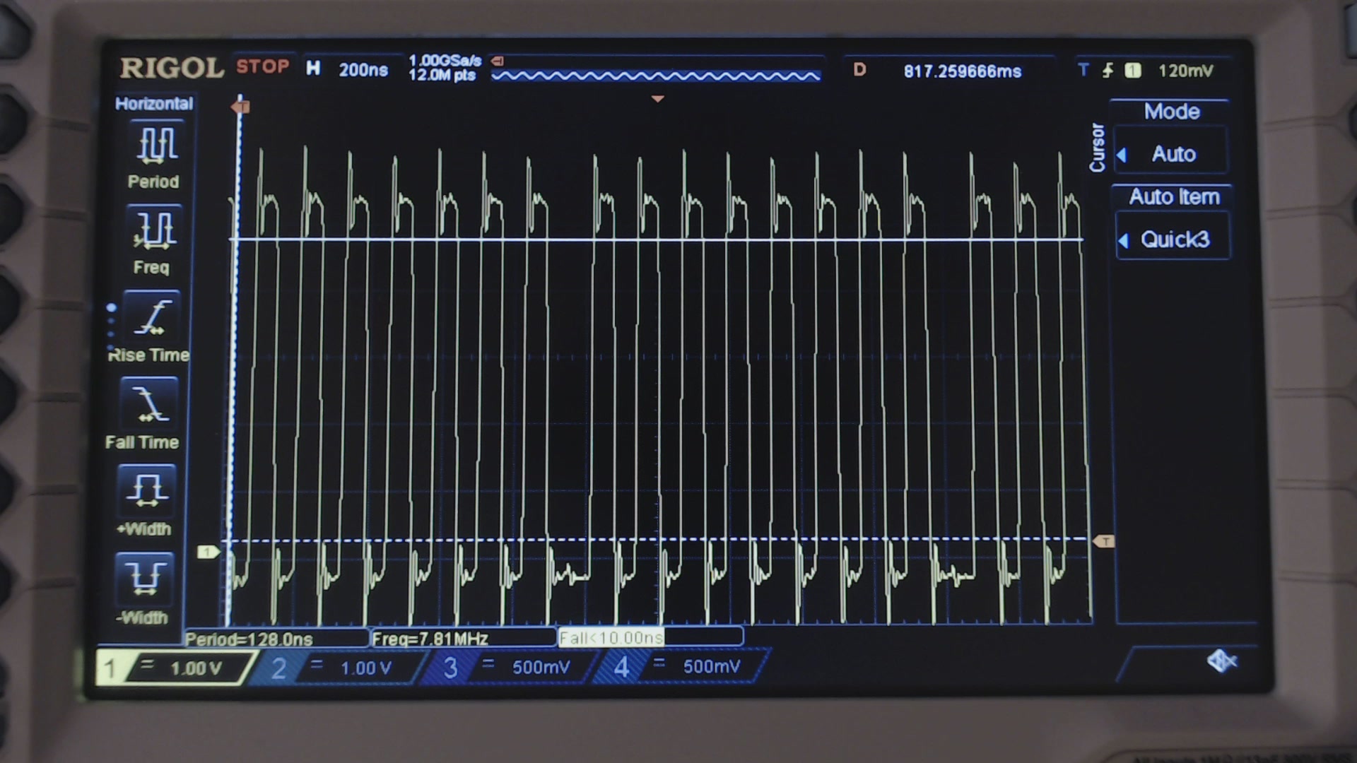
Fig. 2. Clock waveform measured using 16 NOPs on the code shown above.
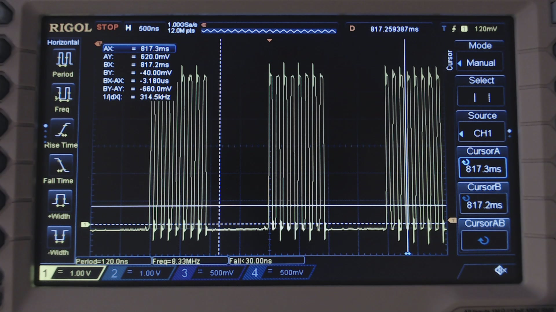
Fig. 2. Clock waveform measured using 15 NOPs on the code shown above. A byte out of two is missing!
This solution has one drawback, with respect to the loop_until_bit_is_set() function: if an interrupt occurs during a transmission, the CPU will always wait 16 cycles, regardless if the SPI already finished sending the previous data (while the interrupt was in execution). With loop_until_bit_is_set() this problem might be partially mitigated, especially, as we’ll see later, when we will use the USART instead.
So now, knowing that we need 17 CPU cycles for each byte, we can determine EXACTLY how many cycles will be employed by the following piece of code, needed to send one character and wait until the SPSR is ready to accept a new byte:
out SPDR, r17; (write data to be sent)
Wait_Transmit: in r16, SPSR; (Load SPSR to register r16)
sbrs r16, SPIF; (SPIF bit set? exit)
rjmp Wait_Transmit; (jump to the first instruction)
Note: in r17 we have the data to be sent.
We know that the SPIF bit will be high 16 cycles after the OUT instruction. So this is the sequence of instructions which are actually executed by the CPU:
| Instruction | Current cycle (before instruction is executed) |
SPIF in SPDR when instruction is executed |
| out | 0 | 1 |
| in | 1 | 0 |
| sbrs | 2 | 0 |
| rjmp (cycle 1) | 3 | 0 |
| rjmp (cycle 2) | 4 | 0 |
| in | 5 | 0 |
| sbrs | 6 | 0 |
| rjmp (cycle 1) | 7 | 0 |
| rjmp (cycle 2) | 8 | 0 |
| in | 9 | 0 |
| sbrs | 10 | 0 |
| rjmp (cycle 1) | 11 | 0 |
| rjmp (cycle 2) | 12 | 0 |
| in | 13 | 0 |
| sbrs | 14 | 0 |
| rjmp (cycle 1) | 15 | 0 |
| in | 16 | 0 |
| sbrs | 17 | 1 |
| rjmp (cycle 1) | 18 | 1 |
| rjmp (cycle 2) | 20 | 1 |
| in | 21 | 1 |
| sbrs * (cycle 1) | 22 | 1 |
| sbrs * (cycle 2) | 23 | 1 |
*Note: In the last step, the sbrs instruction takes 2 cycles, because SPIF is one.
As you can see, it takes 24 cycles (0 through 23) to send 8 bytes of data, instead of 16! That is, you’re sending only at 5.3 Mbps, i.e. 0.67 MBps! Even though this value is closer to what we measured, we are still missing the part in which we actually read the received data from the SPDR register (with an “in” instruction) and we write this value to our buffer (with a “st” instruction), accounting for 3 other cycles. This would yield 590kB/s, still much larger than we actually achieved.
And of course, when reading multiple bytes, we must create a loop and check if we finished reading the required number of bytes, etc.
If you are familiar with the SPI module you can also make clever optimizations, because the SPDR is double buffered in reception. For instance, the pseudo code (which works if you need to send at least 2 bytes) might look like:
SPDR = 0xFF ; after this instruction we have 17 cycles in which we can do something else.
Set remainingBytes to BytesToRead-1
ReceiveLoop:
Wait for SPIF bit set in SPDR register
SPDR = 0xFF
Read SPDR and put into the destination array (Note that SPDR in read and write mode are actually two different registers!)
Decrement RemainingBytes
If remainingBytes > 0
Jump to ReceiveLoop
Endif
Wait For SPIF bit set in SPDR register
Read last byte and put it into the destination array
In C code we get:
SPDR = 0xFF; // after this instruction we have 17 cycles in which we can do something else.
remainingBytes = cnt - 1; // dont worry: the compiler will optimize and won't allocate a new variable!
do
{
loop_until_bit_is_set(SPSR, SPIF); //Wait for SPIF bit set in SPDR register
SPDR = 0xFF;
*p++ = SPDR; //Read SPDR and put into the destination array (Note that SPDR in read and write mode are actually two different registers!)
remainingBytes--; // Decrement remainingBytes
}
while (remainingBytes);
loop_until_bit_is_set(SPSR, SPIF); //Wait for SPIF bit set in SPDR register
*p++ = SPDR; // Read last byte and put it into the destination array
This code is much more optimized, because instead of doing nothing during the transmission, we do a lot of other work: we read the data, we store it into our array, we decrement the counter, we check if there are remaining bytes left and we make the jump to the beginning of the loop.
And the time we get now is 1.86s (495kB/s). Taking into account the 0.4s overhead due to the card delay, we have 1.46s, i.e. 0.63kB/s, which is very close to the 0.67 MB/s that we calculated before (note we still have the other software overhead and the timing previously shown in the table is no longer valid, as we are no more calling “loop_until_bit_is_set” just after writing to SPDR).
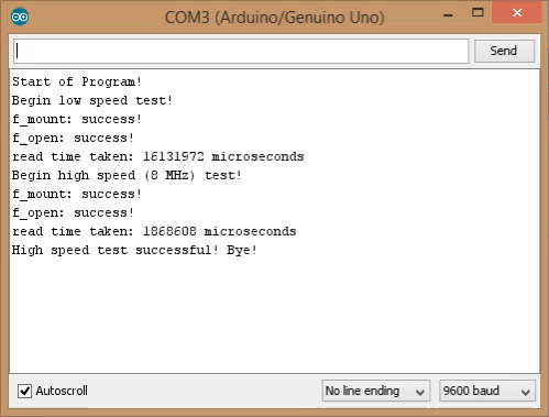
Fig. 4: Serial output of the SPI optimized Code
The scope shows clearly the optimized throughput:
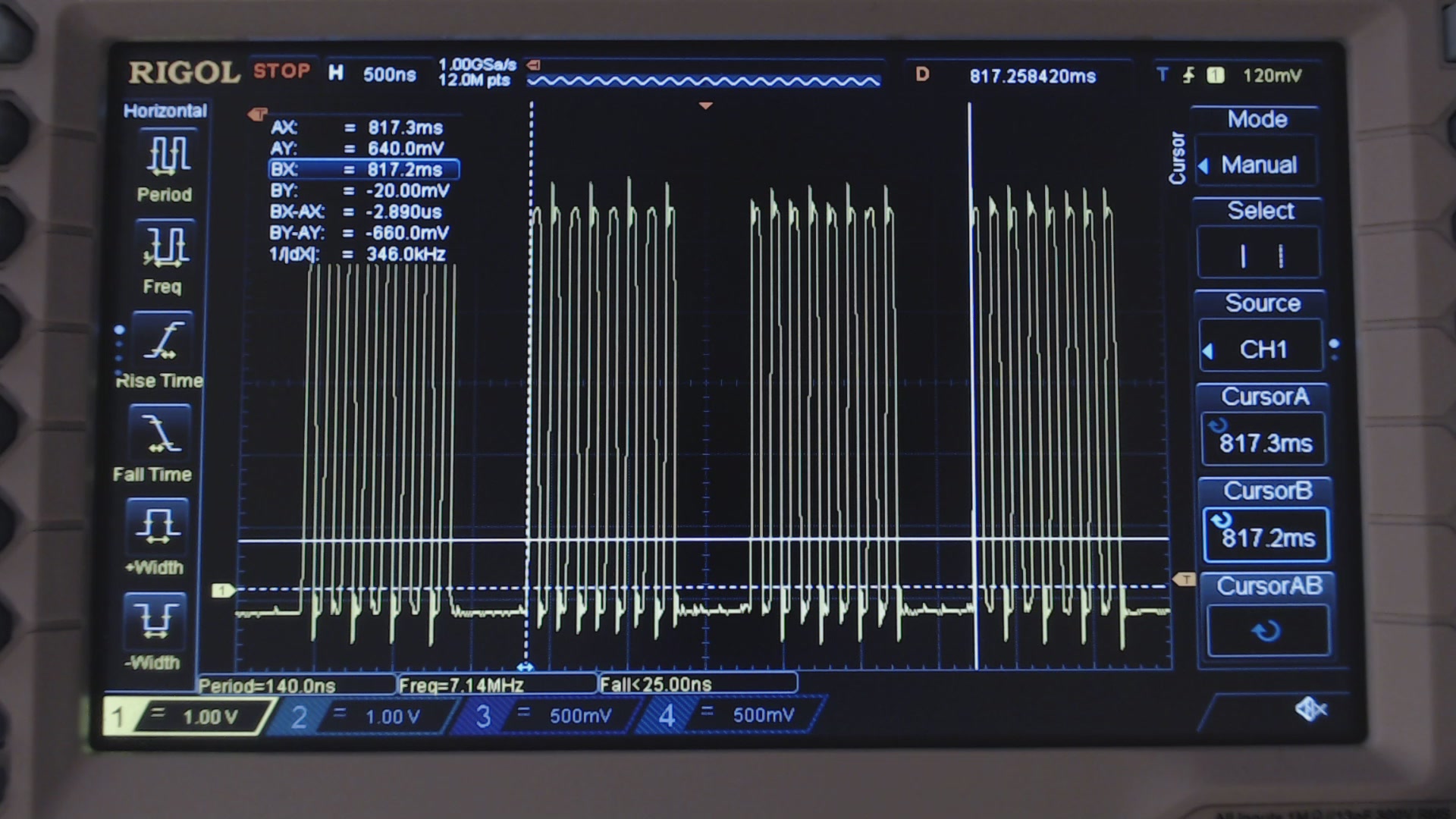
Fig. 5: Clock waveform with optimiyed SPI code.
In fact, two bytes are sent in 2.9 microseconds, that is, 690kB/s. Much better than before, but still not enough. For those who are curious to see the performance of the code of the past episode, here is the measurement with the scope:
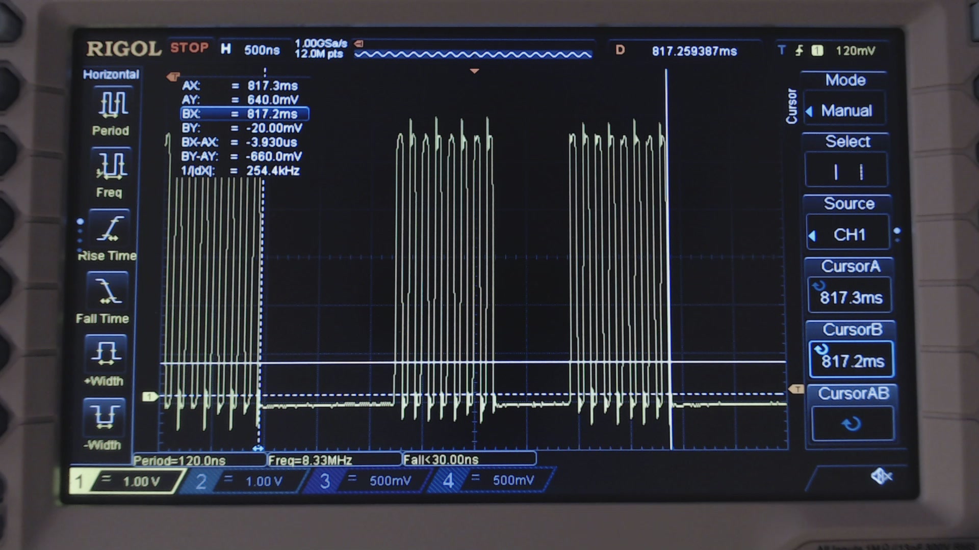
Fig. 6: Clock waveform with the original unoptimized code of the last post.
In Fig 6, we are sending 2 bytes in about 4 microseconds, i.e. 500kB/s. In other words, this code alone was responsible for the loss of HALF of the loss of performances!
The USART in SPI MODE
Luckily, with the USART in SPI mode we can send data without any gap between consecutive bytes.
In fact, the USART has a double buffered transmission (and read) register: i.e. there is a separate transmit register and transmit buffer (the latter is not accessible by the CPU). In other words, we can write fresh data even if the USART is still sending the previous one, provided that the transmit register is empty (i.e. regardless if the transmit buffer is full).
This is very useful, because in this way we can provide the USART module with new data before it is “too late”, and continuous transmission (without gaps) can occur. In fact, when the USART transmits the last bit of the transmit buffer, it seamlessly copy the transmit register to the transmit buffer, so it can proceed (i.e. exactly after the last bit has been outputted) with the first bit of the new data just after the first byte as been sent.
In this way we can safely use the loop_until_bit_is_set() (to check if the transmit register is empty), being sure that there won’t be a transfer gap. In fact, even if the “loop_until_bit_is_set()” might take up to 6 clock cycles (the worst case is when the bit is set just after the first “in” instruction, and this would yield 6 CPU cycles), the USART will be still sending data, and you have 10 other more CPU cycles to write to the transmit buffer, before the transmitter goes idle (i.e. before transmit gap would occur).
Therefore, the C code for sending data becomes:
cnt -= 2; // next two transmissions are performed out of the do…while loop.
UDR0 = 0xFF;
loop_until_bit_is_set(UCSR0A, UDRE0);
UDR0 = 0xFF;
do
{
loop_until_bit_is_set(UCSR0A, RXC0);
*p++ = UDR0;
UDR0 = 0xFF;
cnt--;
} while (cnt);
loop_until_bit_is_set(UCSR0A, RXC0);
*p++ = UDR0;
loop_until_bit_is_set(UCSR0A, RXC0);
UCSR0A |= TXC0;
*p++ = UDR0;
With this new arrangement, there is no gap between bytes as you can see from the scope.
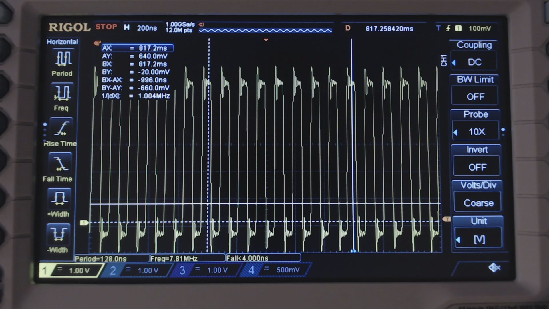
Fig. 7: Clock output with the USART in SPI mode. No gap is generated between bytes!
Furthermore, measuring the delay between the blue LED turning on (yellow trace) and the red LED turning off (blue trace), we get the total time taken by our test program to read the 900kiB file.
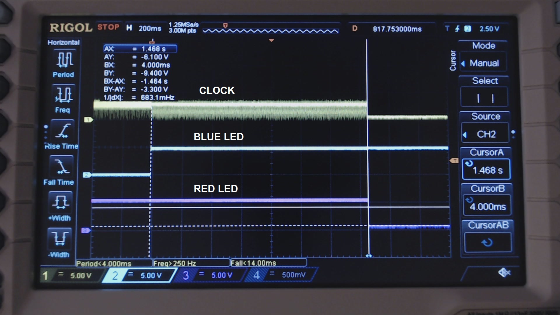
Fig. 8: Measuring the time taken by reading the 900kiB file.
We get 1.47s, i.e. 627kB/s. Taking into account the 0.4 s (which, once again, does not depend on the clock speed, but on the card and the number of sectors read at once), we get 0.86kB/s. This number can be still improved a little bit if we read in larger chunks, we promise!
Of course, this does not come without any drawbacks. In fact, you’ll lose the ability to send data through the UART, which is used by Arduino Uno for the serial USB transmission (in fact now we use a scope to determine the transfer speed) and programming. Therefore you’ll need to disconnect the RXD wire (or the shield you’re using) when you need to reprogram the Arduino.
Another drawback in Arduino Uno is that the ATMEGA328’s USART is connected to the ATMEGA16U8 through 1-kOhm resistors. Therefore some problem might arise (we’ll see this in the next episode), if the ATMEGA16U8 interferes. We will teach you a trick to overcome this issue in the next episode!
Despite all these drawbacks, we have another small advantage! If we don’t use the SPI, we do not need to use the so stupidly misplaced IOH connector (how irritating is the fact that they didn’t place it on a 0.1” grid like the other connectors?!?). We can therefore use normal veroboards for our shields! Good!
Finally, here are the step to replicate our results!
The hack!
Prerequisites
As shown in the previous episode you need a 900kiB (640×480 24 bit) bitmap file named test.bmp in your SD card. You also need the hack of the previous episode and you need the Arduino installed on your system. Of course also you need an Arduino J.
Step 1:
Download the USART test-sd sketch.
Step 2:
Prepare the circuit shown in the schematics below. The breadboard image show a possible arrangement. Pease note that again we used the wires to connect the SD+Display module just to show you that there are resistors! In practice (see actual figure) we put the module over the 1.5k resistors! Please also note that, unlike the previous episode, we have also a fourth 1.5k resistor, connected to the MISO line. This is due because the ATMEGA16U2 (i.e. the uart to USB built in converter) is powered at 5V and its TXD pin is connected to the RXD pin of the ATMEGA328P with a 1k resistor.
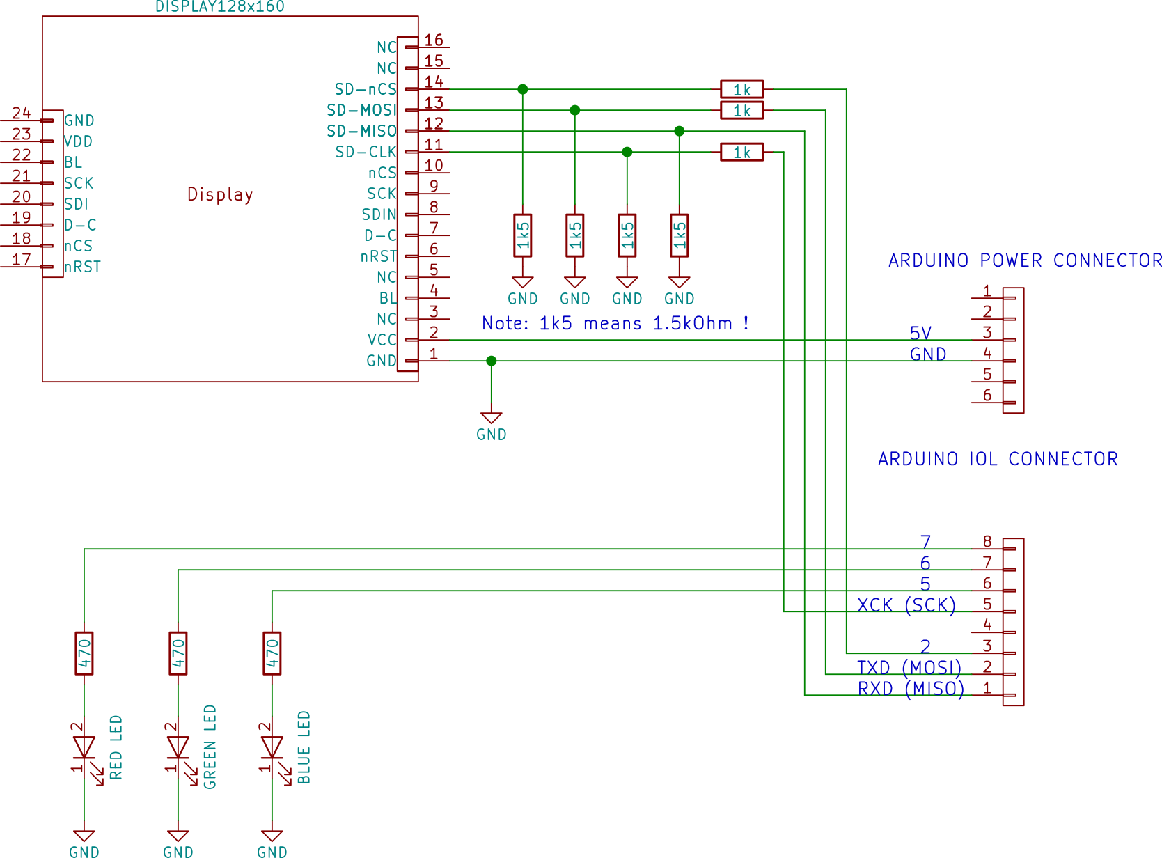
Fig. 9: Schematics of the SD connection to the USART.
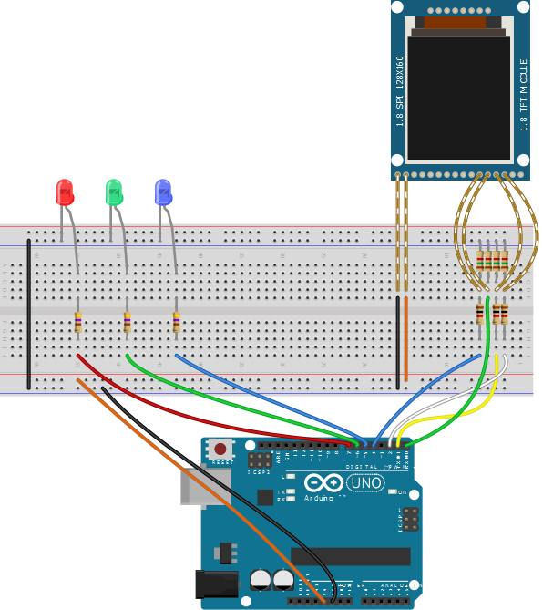
Fig. 10: Example of breadboard layout for the connection of the SD to the USART. The image was created using Fritzing (http://fritzing.org).
This is our actual breadboard implementation.
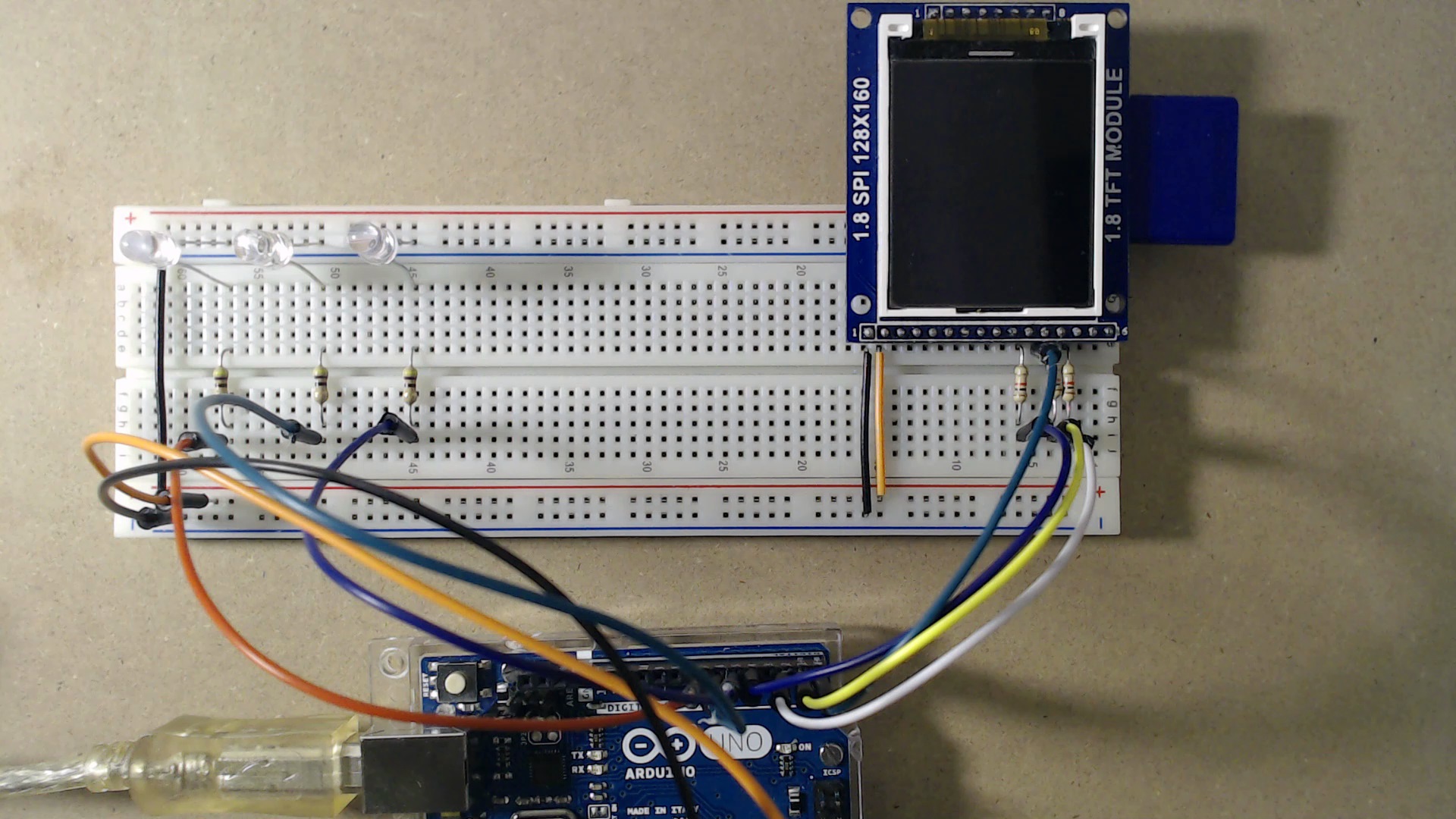
Fig. 11: Actual breadboard implementation.
Step 3:
If you want to measure the time taken by the new program, you have two possibilities: use a two channel scope, and connect one channel to the output connected to the red LED and the other to the output connected to the blue LED. Measure the time between when the blue LED turns on a when the red LED turns off. Otherwise, use a camera/phone and take a video of the LEDs. Use then a program such as virtualDub or AviDemux to analyze (with accuracy depending on your frame rate, tyipically 1/30fps = 33ms) this time!
That’s all for now. Don’t miss the next episode! After all this wait, we will be actually playing the video!!!
Be sure to watch the video of this episode on our youtube channel! Also, rate, comment, share and subscribe!